Download
1 / 42
420 likes | 519 Views
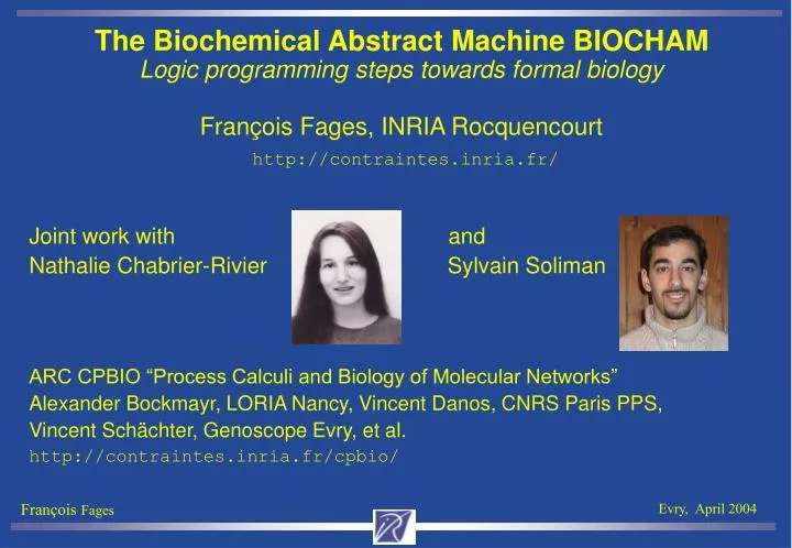
The Biochemical Abstract Machine BIOCHAM Logic programming steps towards formal biology François Fages, INRIA Rocquencourt http://contraintes.inria.fr/. Joint work with and Nathalie Chabrier-Rivier Sylvain Soliman

E N D
The Biochemical Abstract Machine BIOCHAMLogic programming steps towards formal biologyFrançois Fages, INRIA Rocquencourthttp://contraintes.inria.fr/ • Joint work with and • Nathalie Chabrier-Rivier Sylvain Soliman • ARC CPBIO “Process Calculi and Biology of Molecular Networks” • Alexander Bockmayr, LORIA Nancy, Vincent Danos, CNRS Paris PPS, • Vincent Schächter, Genoscope Evry, et al. • http://contraintes.inria.fr/cpbio/
Current Revolution in Systems Biology • Elucidation of high-level biological processes • in terms of their biochemical basis at the molecular level. • Mass production of genomic and post-genomic data: • ARN expression, protein synthesis, protein-protein interactions,… • Need for a strong parallel effort on the formal representation of biological processes: Systems Biology. • Need for formal tools for modeling and reasoning about their global behavior.
Formalisms for Modeling Biochemical Systems • Diagrammatic notation • Boolean networks [Thomas 73] • Milner’s pi–calculus [Regev-Silverman-Shapiro 99-01, Nagasali et al. 00] • Concurrent transition systems [Chabrier-Chiaverini-Danos-Fages-Schachter 03] • Biochemical abstract machine BIOCHAM [Chabrier-Fages-Soliman 03] • Pathway logic [Eker-Knapp-Laderoute-Lincoln-Meseguer-Sonmez 02] • Bio-ambients [Regev-Panina-Silverman-Cardelli-Shapiro 03] • Differential equations • Hybrid Petri nets [Hofestadt-Thelen 98, Matsuno et al. 00] • Hybrid automata [Alur et al. 01, Ghosh-Tomlin 01] • Hybrid concurrent constraint languages [Bockmayr-Courtois 01]
Our Goal • Beyond simulation, provide formal tools for querying, validating and completing biological models. • Our proposal: • Use of temporal logic CTL as a query language for models of biological processes; • Use of concurrent transition systems for their modeling; • Use of symbolic and constraint-based model checkers for automatically evaluating CTL queries in qualitative and quantitative models. • Use of inductive logic programming for learning models • In course, learn and teach bits of biology with logic programs.
References • A wonderful textbook: • Molecular Cell Biology. 5th Edition, 1100 pages+CD, Freeman Publ. • Lodish, Berk, Zipursky, Matsudaira, Baltimore, Darnell. Nov. 2003. • Genes and signals. Ptashne, Gann. CSHL Press. 2002. • Modeling dynamic phenomena in molecular and cellular biology. • Segel. Cambridge Univ. Press. 1987. • Modeling and querying bio-molecular interaction networks. • Chabrier, Chiaverini, Danos, Fages, Schächter. To appear in TCS. 2004. • The biochemical abstract machine BIOCHAM. Chabrier, Fages, Soliman. http://contraintes.inria.fr/BIOCHAM
Plan of the Talk • Introduction • A simple algebra of cell molecules • Concurrent transition systems of biochemical reactions • Example of the mammalian cell cycle control • Temporal logic CTL as a query language • Computational results with BIOCHAM • Learning reaction rules • An experiment with inductive logic programming • Kinetics models • Simulation with differential equations • Hybrid systems • Conclusion
2. A Simple Algebra of Cell Molecules • Small molecules: covalent bonds (outer electrons shared) 50-200 kcal/mol • 70% water • 1% ions • 6% amino acids (20), nucleotides (5), • fats, sugars, ATP, ADP, … • Macromolecules: hydrogen bonds, ionic, hydrophobic, Waals 1-5 kcal/mol • Stability and bindings determined by the number of weak bonds: 3D shape • 20% proteins (50-104 amino acids) • RNA (102-104 nucleotides AGCU) • DNA (102-106 nucleotides AGCT)
Structure Levels of Proteins • 1) Primary structure: word of n amino acids residues (20n possibilities) • linked with C-N bonds • ICLP • Isoleucine Cysteine Leucine Proline • 2) Secondary: word of m a-helix, b-strands, random coils,… (3m-10m) • stabilized by hydrogen bonds H---O • 3) Tertiary 3D structure: spatial folding • stabilized by • hydrophobic • interactions
Formal proteins • Cyclin dependent kinase 1 Cdk1 • (free, inactive) • Complex Cdk1-Cyclin B Cdk1–CycB • (low activity) • Phosphorylated form Cdk1~{thr161}-CycB • at site threonine 161 • (high activity) • (BIOCHAM syntax)
Abstraction of gene expression DNA RNA protein • DNA:word over 4 nucleotides Adenine, Guanine, Cytosine, Thymine • double helix of pairs A--T and C---G • Replication: DNA synthesis • Genes: parts of DNA • Transcription: RNA copying from a gene • #ERCC1-(PRB-JUN-CFOS)
BIOCHAM Algebra of Cell Molecules • E ::= Name|E-E|E~{E,…,E}|(E) S ::= _|E+S • Names: molecules, proteins, #gene binding sites, abstract @processes… • - : binding operator for protein complexes, gene binding sites, … • Associative and commutative. • ~{…}: modification operator for phosphorylated sites, … • Set of modified sites (Associative, Commutative, Idempotent). • + : solution operator, “soup aspect”, Assoc. Comm. Idempotent, Neutral _ • No membranes, no transport formalized. Bitonal calculi [Cardelli 03].
Plan of the talk • Introduction • A simple algebra of cell molecules • Concurrent transition systems of biochemical reactions • Example of the mammalian cell cycle control • Temporal logic CTL as a query language • Computational results with BIOCHAM • Learning reaction rules • An experiment with inductive logic programming • Kinetics models • Simulation with differential equations • Hybrid systems • Conclusion
3. Concurrent Transition Syst. of Biochemical Reactions • Enzymatic reactions: • R ::= S=>S | S=[E]=>S | S=[R]=>S | S<=>S | S<=[E]=>S • (where A<=>B stands for A=>BB=>A and A=[C]=>B for A+C=>B+C, etc.) • define a concurrent transition system over integers denoting the multiplicity of the molecules (multiset rewriting). • One can associate a finite abstract CTS over booleanstate variables denoting the presence/absence of molecules • which correctly over-approximates the set of all possible behaviors • a reaction A+B=>C+D is translated with 4 rules for possible consumption: • A+BA+B+C+D A+BA+B +C+D • A+BA+B+C+D A+BA+B+C+D
Six Rule Schemas • Complexation: A + B => A-B Decomplexation A-B => A + B • Cdk1+CycB => Cdk1–CycB • Phosphorylation: A =[C]=> A~{p} Dephosphorylation A~{p} =[C]=> A • Cdk1–CycB =[Myt1]=> Cdk1~{thr161}-CycB • Cdk1~{thr14,tyr15}-CycB =[Cdc25~{Nterm}]=> Cdk1-CycB • Synthesis: _ =[C]=> A. • _ =[#Ge2-E2f13-Dp12]=> CycA • Degradation: A =[C]=> _. • CycE =[@UbiPro]=> _ (not for CycE-Cdk2 which is stable)
MAPK Signaling Pathway • RAF + RAFK <=> RAF-RAFK. • RAF~{p1} + RAFPH <=> RAF~{p1}-RAFPH. • MEK~$P + RAF~{p1} <=> MEK~$P-RAF~{p1} • where p2 not in $P. • MEKPH + MEK~{p1}~$P <=> MEK~{p1}~$P-MEKPH. • MAPK~$P + MEK~{p1,p2} <=> MAPK~$P-MEK~{p1,p2} • where p2 not in $P. • MAPKPH + MAPK~{p1}~$P <=> MAPK~{p1}~$P-MAPKPH. • RAF-RAFK => RAFK + RAF~{p1}. • RAF~{p1}-RAFPH => RAF + RAFPH. • MEK~{p1}-RAF~{p1} => MEK~{p1,p2} + RAF~{p1}. • MEK-RAF~{p1} => MEK~{p1} + RAF~{p1}. • MEK~{p1}-MEKPH => MEK + MEKPH. • MEK~{p1,p2}-MEKPH => MEK~{p1} + MEKPH. • MAPK-MEK~{p1,p2} => MAPK~{p1} + MEK~{p1,p2}. • MAPK~{p1}-MEK~{p1,p2} => MAPK~{p1,p2}+ MEK~{p1,p2}. • MAPK~{p1}-MAPKPH => MAPK + MAPKPH. • MAPK~{p1,p2}-MAPKPH => MAPK~{p1} + MAPKPH.
MAPK Signaling Pathway • RAF + RAFK <=> RAF-RAFK. • RAF~{p1} + RAFPH <=> RAF~{p1}-RAFPH. • MEK~$P + RAF~{p1} <=> MEK~$P-RAF~{p1} • where p2 not in $P. • MEKPH + MEK~{p1}~$P <=> MEK~{p1}~$P-MEKPH. • MAPK~$P + MEK~{p1,p2} <=> MAPK~$P-MEK~{p1,p2} • where p2 not in $P. • MAPKPH + MAPK~{p1}~$P <=> MAPK~{p1}~$P-MAPKPH. • RAF-RAFK => RAFK + RAF~{p1}. • RAF~{p1}-RAFPH => RAF + RAFPH. • MEK~{p1}-RAF~{p1} => MEK~{p1,p2} + RAF~{p1}. • MEK-RAF~{p1} => MEK~{p1} + RAF~{p1}. • MEK~{p1}-MEKPH => MEK + MEKPH. • MEK~{p1,p2}-MEKPH => MEK~{p1} + MEKPH. • MAPK-MEK~{p1,p2} => MAPK~{p1} + MEK~{p1,p2}. • MAPK~{p1}-MEK~{p1,p2} => MAPK~{p1,p2}+ MEK~{p1,p2}. • MAPK~{p1}-MAPKPH => MAPK + MAPKPH. • MAPK~{p1,p2}-MAPKPH => MAPK~{p1} + MAPKPH.
Cell Cycle: G1 DNA Synthesis G2 Mitosis • G1: CdK4-CycD • Cdk6-CycD • Cdk2-CycE • S: Cdk2-CycA • G2 • M: Cdk1-CycA • Cdk1-CycB
Kohn’s map detail for Cdk2 • Complexation with CycA and CycE • Phosphorylation sites PY15 and P • Biocham Rules: • cdk2~$P + cycA-$C => cdk2~$P-cycA-$C • where $C in {_,cks1} . • cdk2~$P + cycE~$Q-$C => cdk2~$P-cycE~$Q-$C • where $C in {_,cks1} . • p57 + cdk2~$P-cycA-$C => p57-cdk2~$P-cycA-$C • where $C in {_, cks1}. • cycE-$C =[cdk2~{p2}-cycE-$S]=> cycE~{T380}-$C • where $S in {_, cks1} and $C in {_, cdk2~?, cdk2~?-cks1} • 147-2733 rules, 165 proteins and genes, 500 variables, 2500 states.
Plan of the talk • Introduction • A simple algebra of cell molecules • Concurrent transition systems of biochemical reactions • Example of the mammalian cell cycle control • Temporal logic CTL as a query language • Expressivity and computational results • Learning reaction rules • An experiment with inductive logic programming • Kinetics models • Simulation with differential equations • Hybrid systems • Conclusion
E, A Non-determinism AG EU EF F,G,U Time 4. Temporal Logic CTL as a Query Language • Computation Tree Logic
Kripke Structures • A Kripke structure K is a triple (S; R; L) where S is a set of states, and RSxS is a total relation. • s |= f if f is true in s, • s |= E f if there is a path from s such that |= f, • s |= A f if for every path from s, |= f, • |= f if s |= f where s is the starting state of , • |= X f if 1 |= f, • |= F f if there exists k >0 such that k |= f, • |= G f if for every k >0, k |= f, • |= f1 U f2 iff there exists k>0 such that k |= f for all j < k j |= f. • Following [Emerson 90] we identify a formula f to the set of states which satisfy it f ~ {sS : s |= f}.
Symbolic Model Checking • Model Checking is an algorithm for computing, in a given finite Kripke structure the set of states satisfying a CTL formula: {sS : s |= f}. • Basic algorithm: represent K as a graph and iteratively label the nodes with the subformulas of f which are true in that node. • Add f to the states satisfying f • Add EF f(EX f) to the (immediate) predecessors of states labeled by f • Add E(f1 U f2 ) to the predecessor states of f2 while they satisfy f1 • Add EG f to the states for which there exists a path leading to a non trivial strongly connected component of the subgraph of states satisfying f • Symbolic model checking: use OBDDs to represent states and transitions as boolean formulas (S is finite).
Biological Queries (1/3) • About reachability: • Given an initial state init, can the cell produce some protein P? init EF(P) • Which are the states from which a set of products P1,. . . , Pn can be produced simultaneously? EF(P1^…^Pn) • About pathways: • Can the cell reach a state s while passing by another state s2? init EF(s2^EFs) • Is state s2 a necessary checkpoint for reaching state s? EF(s2U s) • Is it possible to produce P without using nor creating Q? EF(Q U s) • Can the cell reach a state s without violating some constraints c? init EF(c U s)
Biological Queries (2/3) • About stability: • Is a certain (partially described) state s a stable state? sAG(s)sAG(s) (s denotes both the state and the formula describing it). • Is s a steady state (with possibility of escaping) ? sEG(s) • Can the cell reach a stable state? initEF(AG(s))not a LTL formula. • Must the cell reach a stable state? initAF(AG(s)) • What are the stable states? Not expressible in CTL [Chan 00]. • Can the system exhibit a cyclic behavior w.r.t. the presence of P ? init EG((P EF P) ^ (P EF P))
Biological Queries (3/3) • About the correctness of the model: • Can one see the inaccuracies of the model and correct them? • Exhibit a counterexample pathway or a witness. Suggest refinements of the model or biological experiments to validate/invalidate the property of the model. • About durations: • How long does it take for a molecule to become activated? • In a given time, how many Cyclins A can be accumulated? • What is the duration of a given cell cycle’s phase? • CTL operators abstract from durations. Time intervals can be modeled in FO by adding numerical arguments for start times and durations.
MAPK Signaling Pathway • RAF + RAFK <=> RAF-RAFK. • RAF~{p1} + RAFPH <=> RAF~{p1}-RAFPH. • MEK~$P + RAF~{p1} <=> MEK~$P-RAF~{p1} • where p2 not in $P. • MEKPH + MEK~{p1}~$P <=> MEK~{p1}~$P-MEKPH. • MAPK~$P + MEK~{p1,p2} <=> MAPK~$P-MEK~{p1,p2} • where p2 not in $P. • MAPKPH + MAPK~{p1}~$P <=> MAPK~{p1}~$P-MAPKPH. • RAF-RAFK => RAFK + RAF~{p1}. • RAF~{p1}-RAFPH => RAF + RAFPH. • MEK~{p1}-RAF~{p1} => MEK~{p1,p2} + RAF~{p1}. • MEK-RAF~{p1} => MEK~{p1} + RAF~{p1}. • MEK~{p1}-MEKPH => MEK + MEKPH. • MEK~{p1,p2}-MEKPH => MEK~{p1} + MEKPH. • MAPK-MEK~{p1,p2} => MAPK~{p1} + MEK~{p1,p2}. • MAPK~{p1}-MEK~{p1,p2} => MAPK~{p1,p2}+ MEK~{p1,p2}. • MAPK~{p1}-MAPKPH => MAPK + MAPKPH. • MAPK~{p1,p2}-MAPKPH => MAPK~{p1} + MAPKPH.
MAPK Signaling Pathway • MEK~{p1} is a checkpoint for producing MAPK~{p1,p2} • biocham: !E(!MEK~{p1} U MAPK~{p1,p2}) • True • The PH complexes are not compulsory for the cascade • biocham: !E(!MEK~{p1}-MEKPH U MAPK~{p1,p2}) • false • Step 1 rule 15 • Step 2 rule 1 RAF-RAFK present • Step 3 rule 21 RAF~{p1} present • Step 4 rule 5 MEK-RAF~{p1} present • Step 5 rule 24 MEK~{p1} present • Step 6 rule 7 MEK~{p1}-RAF~{p1} present • Step 7 rule 23 MEK~{p1,p2} present • Step 8 rule 13 MAPK-MEK~{p1,p2} present • Step 9 rule 27 MAPK~{p1} present • Step 10 rule 15 MAPK~{p1}-MEK~{p1,p2} present • Step 11 rule 28 MAPK~{p1,p2} present
Mammalian Cell Cycle Control Benchmark • 700 rules, 165 proteins and genes, 500 variables, 2500 states. • BIOCHAM NuSMV model-checker time in seconds:
Plan of the talk • Introduction • A simple algebra of cell molecules • Concurrent transition systems of biochemical reactions • Example of the mammalian cell cycle control • Temporal logic CTL as a query language • Computational results with BIOCHAM • Learning reaction rules • An experiment with inductive logic programming • Kinetics models • Simulation with differential equations • Hybrid systems • Conclusion
5. Learning Reaction Weights and Rules • Idea 1: learning reaction weights from temporal properties • reaction weights restricts the non-determinism (Markov models) • Idea 2: learn reaction rules from temporal properties of the system. • Learning of cell cycle reaction rules from reachability properties and counterexamples with Progol [Muggleton 00]. • reaction([m_CP,m_Y],[m_pM]). • reaction([m_CP],[m_C2]). • % reaction([m_pM],[m_M]). • reaction([m_M],[m_C2,m_YP]). • reaction([m_C2],[m_CP]). • reaction([m_YP],[]). • reaction([],[m_Y]). • pathway(S1,S2) :- same(S1,S2). • pathway(S1,S2) :- reaction(L1,L2), transition(S1,L1,S3,L2), pathway(S3,S2).
Inductive Logic Programming • reaction([m_pM],[m_M]) learned… • 6th PCRD APRIL 2 “Applications of Probabilistic Inductive Logic Progr.” Luc de Raedt, Univ. Freiburg, Stephen Muggleton, Imperial College London.
Plan of the talk • Introduction • A simple algebra of cell molecules • Concurrent transition systems of biochemical reactions • Example of the mammalian cell cycle control • Temporal logic CTL as a query language • Computational results with BIOCHAM • Learning reaction rules • An experiment with inductive logic programming • Kinetics models • Simulation with differential equations • Hybrid system • Conclusion
6. Kinetics Models • Enzymatic reactions with rates k1 k2 k3 • E+S k1 C k2 E+P • E+S k3 C • can be compiled by the law of mass action into a system of • Michaelis-Menten Ordinary Differential Equations (non-linear) • dE/dt = -k1ES+(k2+k3)C • dS/dt = -k1ES+k3C • dC/dt = k1ES-(k2+k3)C • dP/dt = k2C
Gene Interaction Networks • Gene interaction example [Bockmayr-Courtois 01] • Hybrid Concurrent Constraint Programming HCC [Saraswat et al.] • 2 genes x and y. • Hybrid linear approximation • dx/dt = 0.01 – 0.02*x if y < 0.8 • dx/dt = – 0.02*x if y ≥ 0.8 • dy/dt = 0.01*x
Concurrent Transition System • Time discretization using Euler’s method: • y < 0.8 x’ = x + dt*(0.01-0.02*x) , y’ = y + dt*0.01*x • y ≥ 0.8 x’ = x + dt*(0.01-0.02*x) , y’ = y + dt*0.01*x • Initial condition: x=0, y=0. • Translation into a CLP(R) program (dt=1) • Init :- X=0, Y=0, p(X,Y). • p(X,Y):-X>=0, Y>=0, Y<0.8, • X1=X-0.02*X+0.01, Y1=Y+0.01*X, p(X1,Y1). • p(X,Y):-X>=0, Y>=0, Y>=0.8, • X1=X-0.02*X, Y1=Y+0.01*X, p(X1,Y1).
Proving CTL properties by computing fixpoints of Constraint Logic Programs Theorem [Delzanno Podelski 99] EF(f)=lfp(TP{p(x):-f}), EG(f)=gfp(TPf ). Safety property AG(f) iff EF(f) iff initlfp(TP{f}) Liveness property AG(f1AF(f2)) iff initlfp(TPf1gfp(T P{f2} ) ) Implementation in Sicstus-Prolog CLP(R,B) [Delzanno 00]
Deductive Model Checker DMC: Gene Interaction • r(init, p(s_s,A,B), {A=0,B=0}). • r(p(s_s,A,B), p(s_s,C,D), {A>=0,B>=0.8,C=A-0.02*A,D=B+0.01*A}). • r(p(s_s,A,B), p(s_s,C,D), {A>=0,B>=0,B<0.8, • C=A-0.02*A+0.01,D=B+0.01*A}). • | ?- prop(P,S). • P = unsafe, S = p:s*(x>=0.6) • | ?- ti. • Property satisfied. Execution time 0.0 • | ?- ls. • s(0, p(s_s,A,_), {A>=0.6}, 1, (0,0)).
Demonstration DMC (continued) • | ?- prop(P,S). • P = unsafe, S = p:s*(x>=0.2) ? • | ?- ti. • Property NOT satisfied. Execution time 1.5 • | ?- ls. • s(0, p(s_s,A,_), {A>=0.2}, 1, (0,0)). • s(1, p(s_s,A,B), {B<0.8,B>=-0.0,A>=0.19387755102040816}, 2, (2,1)). • … • s(26, p(s_s,A,B), {B>=0.0,A>=0.0, • B+0.1982676351105516*A<0.7741338175552753}, 27, (2,26)). • s(27, init, {}, 28, (1,27)).
Conclusion • The biochemical abstract machine BIOCHAM provides: • A first-order-rule-based language for modeling biochemical systems • A powerful query language based on temporal logic CTL • Models of complex biochemical processes, • intracellular and extracellular signaling, • cell-cycle control,… • a repository of models http://contraintes.inria.fr/CMBSlib • Implementation in Prolog + model-checkers NuSMV and DMC • Learning techniques investigated in APrIL 2 • PILP-based learning of reaction weights from temporal properties • PILP-based learning of reaction rules from temporal properties
Perspectives • Collaboration with biologists on BIOCHAM models of the cell-cycle control • Colon cancer therapies, Domenjoud, UHP Nancy • Chronotherapies, Clairambault, INSERM • Hybrid concurrent constraint logic programming[Bockmayr Courtois 01, Saraswat 04] • Multi-scale molecular-electro-physiological models[Sorine et al. 03] • http://www-rocq.inria.fr/sosso/icema2 • http://www.sci.sdsu.edu/movies