Download
1 / 47
470 likes | 588 Views
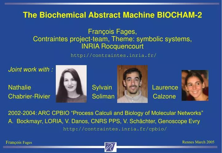
The Biochemical Abstract Machine BIOCHAM-2 François Fages, Contraintes project-team, Theme: symbolic systems, INRIA Rocquencourt http://contraintes.inria.fr/. Joint work with : Nathalie Sylvain Laurence

E N D
The Biochemical Abstract Machine BIOCHAM-2François Fages, Contraintes project-team, Theme: symbolic systems, INRIA Rocquencourthttp://contraintes.inria.fr/ • Joint work with : • Nathalie Sylvain Laurence • Chabrier-Rivier Soliman Calzone • 2002-2004: ARC CPBIO “Process Calculi and Biology of Molecular Networks” • Bockmayr, LORIA, V. Danos, CNRS PPS, V. Schächter, Genoscope Evry • http://contraintes.inria.fr/cpbio/
Systems Biology ? • Multidisciplinary field aiming at getting over the complexity walls to reason about biological processes at the system level. • Virtual cell: emulate high-level biological processes in terms of their biochemical basis at the molecular level (in silico experiments) • Beyond providing tools to biologists, Computer Science has much to offer in terms of concepts and methods. • Bioinformatics: end 90’s, genomic sequences post-genomic data (ARN expression, protein synthesis, protein-protein interactions,… ) • Need for a strong parallel effort on: • - the formal representation of biological processes, • - formal tools for modeling and reasoning about their global behavior.
Language Approach to (Cell) Systems Biology • Qualitative models:from diagrammatic notation to • Boolean networks [Thomas 73] • Milner’s π–calculus [Regev-Silverman-Shapiro 99-01, Nagasali et al. 00] • Concurrent transition systems[Chabrier-Chiaverini-Danos-Fages-Schachter 03] • Biochemical abstract machine BIOCHAM-1[Chabrier-Fages 03] • Pathway logic [Eker-Knapp-Laderoute-Lincoln-Meseguer-Sonmez 02] • Bio-ambients [Regev-Panina-Silverman-Cardelli-Shapiro 03] • Quantitative models: from differential equation systems to • Hybrid Petri nets [Hofestadt-Thelen 98, Matsuno et al. 00] • Hybrid automata [Alur et al. 01, Ghosh-Tomlin 01] • Hybrid concurrent constraint languages [Bockmayr-Courtois 01] • Rule-based compositional language BIOCHAM-2[Chabrier-Fages-Soliman 04]
Plan for today • Introduction • BIOCHAM Language for Modeling Biochemical Systems • Syntax: molecules and reactions • Semantics at 3 abstraction levels: molecule populations, concentrations, Boolean • BIOCHAM Language for Formalizing Biological Properties • Computation Tree Logic for Boolean semantics • Constraint Linear Time Logic for concentration semantics • Machine Learning from Temporal Properties • Learning reaction rules • Learning kinetic parameter values • Conclusion, collaborations and perspectives
2. Modeling Biochemical Systems: syntax of molecules • Small molecules: covalent bonds (outer electrons shared) 50-200 kcal/mol • 70% water • 1% ions • 6% amino acids (20), nucleotides (5), • fats, sugars, ATP, ADP, … • Macromolecules: hydrogen bonds, ionic, hydrophobic, Waals 1-5 kcal/mol • Stability and bindings determined by the number of weak bonds: 3D shape • 20% proteins (50-104 amino acids) • RNA (102-104 nucleotides AGCU) • DNA (102-106 nucleotides AGCT)
Formal proteins • Cyclin dependent kinase 1 Cdk1 • (free, inactive) • Complex Cdk1-Cyclin B Cdk1–CycB • (low activity) • Phosphorylated form Cdk1~{thr161}-CycB • at site threonine 161 • (high activity) • (BIOCHAM syntax)
Formal Genes and RNA • Genes = parts of DNA #ERCC1 • Gene transcription: RNA copying from a gene • RNA expression: Protein synthesis from an RNA • #ERCC1-(PRB-JUN-CFOS)
BIOCHAM Syntax of Molecules • E ::= Name|E-E|E~{E,…,E}|(E) S ::= _|E+S • Names: molecules, proteins, #gene binding sites, abstract @processes… • - : binding operator for protein complexes, gene binding sites, … • Associative and commutative. • ~{…}: modification operator for phosphorylated sites, … • Set of modified sites (Associative, Commutative, Idempotent). • + : solution operator, “soup aspect”, Assoc. Comm. Idempotent, Neutral _ • No membranes, no transport formalized. Bitonal calculi [Cardelli 03].
BIOCHAM Syntax of Reactions • N ::= name : expr for R | • name : R | expr for R | R • R ::= S=>S | S=[E]=>S | • S=[R]=>S | S<=>S | S<=[E]=>S • where A<=>B stands for A=>B and B=>A • A=[C]=>B for A+C=>B+C, etc. • Three abstraction levels: • Boolean abstraction: presence/absence of molecules • Concurrent Transition System • Concentrations: number / volume • ODE • Population of molecules: number of molecules • Multiset Rewriting, Stochastic
Boolean Semantics (BIOCHAM-1) • Associate: • Booleanstate variables to molecules • denoting the presence/absence of molecules in the cell or compartment • A Finite concurrent transition system [Shankar 93] to rules (asynchronous) over-approximating the set of all possible behaviors • A reaction A+B=>C+D is translated with 4 transition rules taking into account the possible consumption of reactants: • A+BA+B+C+D • A+BA+B +C+D • A+BA+B+C+D • A+BA+B+C+D
Six Elementary Reaction Rule Schemas • Complexation: A + B => A-B Decomplexation A-B => A + B • Cdk1+CycB => Cdk1–CycB • Phosphorylation: A =[C]=> A~{p} Dephosphorylation A~{p} =[C]=> A • Cdk1–CycB =[Myt1]=> Cdk1~{thr161}-CycB • Cdk1~{thr14,tyr15}-CycB =[Cdc25~{Nterm}]=> Cdk1-CycB • Synthesis: _ =[C]=> A. • _ =[#Ge2-E2f13-Dp12]=> CycA • Degradation: A =[C]=> _. • CycE =[@UbiPro]=> _ (not for CycE-Cdk2 which is stable)
MAPK Signaling Pathway • RAF + RAFK <=> RAF-RAFK. • RAF~{p1} + RAFPH <=> RAF~{p1}-RAFPH. • MEK~$P + RAF~{p1} <=> MEK~$P-RAF~{p1} • where p2 not in $P. • MEKPH + MEK~{p1}~$P <=> MEK~{p1}~$P-MEKPH. • MAPK~$P + MEK~{p1,p2} <=> MAPK~$P-MEK~{p1,p2} • where p2 not in $P. • MAPKPH + MAPK~{p1}~$P <=> MAPK~{p1}~$P-MAPKPH. • RAF-RAFK => RAFK + RAF~{p1}. • RAF~{p1}-RAFPH => RAF + RAFPH. • MEK~{p1}-RAF~{p1} => MEK~{p1,p2} + RAF~{p1}. • MEK-RAF~{p1} => MEK~{p1} + RAF~{p1}. • MEK~{p1}-MEKPH => MEK + MEKPH. • MEK~{p1,p2}-MEKPH => MEK~{p1} + MEKPH. • MAPK-MEK~{p1,p2} => MAPK~{p1} + MEK~{p1,p2}. • MAPK~{p1}-MEK~{p1,p2} => MAPK~{p1,p2}+ MEK~{p1,p2}. • MAPK~{p1}-MAPKPH => MAPK + MAPKPH. • MAPK~{p1,p2}-MAPKPH => MAPK~{p1} + MAPKPH.
MAPK Signaling Pathway • RAF + RAFK <=> RAF-RAFK. • RAF~{p1} + RAFPH <=> RAF~{p1}-RAFPH. • MEK~$P + RAF~{p1} <=> MEK~$P-RAF~{p1} • where p2 not in $P. • MEKPH + MEK~{p1}~$P <=> MEK~{p1}~$P-MEKPH. • MAPK~$P + MEK~{p1,p2} <=> MAPK~$P-MEK~{p1,p2} • where p2 not in $P. • MAPKPH + MAPK~{p1}~$P <=> MAPK~{p1}~$P-MAPKPH. • RAF-RAFK => RAFK + RAF~{p1}. • RAF~{p1}-RAFPH => RAF + RAFPH. • MEK~{p1}-RAF~{p1} => MEK~{p1,p2} + RAF~{p1}. • MEK-RAF~{p1} => MEK~{p1} + RAF~{p1}. • MEK~{p1}-MEKPH => MEK + MEKPH. • MEK~{p1,p2}-MEKPH => MEK~{p1} + MEKPH. • MAPK-MEK~{p1,p2} => MAPK~{p1} + MEK~{p1,p2}. • MAPK~{p1}-MEK~{p1,p2} => MAPK~{p1,p2}+ MEK~{p1,p2}. • MAPK~{p1}-MAPKPH => MAPK + MAPKPH. • MAPK~{p1,p2}-MAPKPH => MAPK~{p1} + MAPKPH.
2.2 Concentration Semantics • Add kinetic expressions to BIOCHAM reaction rules • k*[A]*[B] for A + B => C • Associate real values to molecules • [A] concentration of A • Associate a system of ordinary differential equations (ODE) • to a system of reaction rules (BIOCHAM model)
Physical Interpretation of Kinetic Expressions • Probability of collision • Different diffusion speeds of molecules (small>substrates>enzymes…) • Average travel in a random walk: 1 μm in 1s, 2μm in 4s, 10μm in 100s • 500000 random collisions per second for a substrate concentration of 10-5 • 50000 random collisions per second for a substrate concentration of 10-6 • 2) Probability of reactionupon collision • non elastic collision determined by the • shape and orientation of matching surfaces • 3) Energy of bonds (for dissociation rates)
The Law of Mass Action is Compositional • Law: The number of reactions is proportional to the number of A and B’s. • A + B k C • reaction rate=kAB=dC/dt , dA/dt=-kAB, dB/dt=-kAB • Diffusion assumption: each molecule moves independently of other molecules in a random walk (dilute solutions, low concentration ). • The dynamics of a complex system is the composition of the dynamics of the reactions under mass action law (at given temperature, pH,…): • E+S k1 C k2 E+P • E+S k3 C • dE/dt = -k1ES+(k2+k3)C dC/dt = k1ES-(k2+k3)C • dS/dt = -k1ES+k3C dP/dt = k2C
Multi-Scale Phenomena Hydrolysis of benzoyl-L-arginine ethyl ester by trypsin present(En,1e-8). present(S,1e-5). absent(C). absent(P). (k1*[En]*[S],km1*[C]) for En+S <=> C. k2*[C] for C => En+P. parameter(k1,4e6). parameter(km1,25). parameter(k2,15). Complex formation 5e-9 in 0.1s Product formation 1e-5 in 1000s
Michaelis-Menten, Hill,… kinetics are not compositional • They are derived from mass action law by quasi-steady approximation for given simple systems: • Simple enzymatic reaction for Michaelis Menten • Simple cooperative n-dimeric enzymatic reaction for Hill of order n • The quasi-steady state approximation may be no longer valid after composition with other molecules and reactions. • In a compositional approach to Systems Biology (making models composable and re-usable in different contexts) • Michaelis-Menten kinetics, Hill kinetics etc. should be abandonned as reaction kinetics (no intrinsic value) and recovered after composition (property of the system)
Plan • Introduction • BIOCHAM Language for Modeling Biochemical Systems • Syntax • Semantics at 3 abstraction levels (molecule populations, concentrations, Boolean) • BIOCHAM Language for Formalizing Biological Properties • Computation Tree Logic for Boolean semantics • Constraint Linear Time Logic for concentration semantics • Machine Learning from Temporal Properties • Learning reaction rules • Learning kinetic parameter values • Conclusion, collaborations and perspectives
E, A Non-determinism AG EU EF F,G,U Time 3. Temporal Logic CTL as a Query Language • Computation Tree Logic [Clarke & al. 99]
Biological Queries (1/3) • About reachability: • Given an initial state init, can the cell produce some protein P? init EF(P) • Which are the states from which a set of products P1,. . . , Pn can be produced simultaneously? EF(P1^…^Pn) • About pathways: • Can the cell reach a state s while passing by another state s2? init EF(s2^EFs) • Is state s2 a necessary checkpoint for reaching state s? EF(s2U s) • Is it possible to produce P without using nor creating Q? EF(Q U s) • Can the cell reach a state s without violating some constraints c? init EF(c U s)
Biological Queries (2/3) • About stability: • Is a certain (partially described) state s a stable state? sAG(s)sAG(s) (s denotes both the state and the formula describing it). • Is s a steady state (with possibility of escaping) ? sEG(s) • Can the cell reach a stable state? initEF(AG(s))not a LTL formula. • Must the cell reach a stable state? initAF(AG(s)) • What are the stable states? Not expressible in CTL [Chan 00]. • Can the system exhibit a cyclic behavior w.r.t. the presence of P ? init EG((P EF P) ^ (P EF P))
Biological Queries (3/3) • About the correctness of the model: • Can one see the inaccuracies of the model and correct them? • Exhibit a counterexample pathway or a witness. Suggest refinements of the model or biological experiments to validate/invalidate the property of the model. • About durations: • How long does it take for a molecule to become activated? • In a given time, how many Cyclins A can be accumulated? • What is the duration of a given cell cycle’s phase? • CTL operators abstract from durations. Time intervals can be modeled in FO by adding numerical arguments for start times and durations.
MAPK Signaling Pathway • MEK~{p1} is a checkpoint for producing MAPK~{p1,p2} • biocham: !E(!MEK~{p1} U MAPK~{p1,p2}) • True • The PH complexes are not compulsory for the cascade • biocham: !E(!MEK~{p1}-MEKPH U MAPK~{p1,p2}) • false • Step 1 rule 15 • Step 2 rule 1 RAF-RAFK present • Step 3 rule 21 RAF~{p1} present • Step 4 rule 5 MEK-RAF~{p1} present • Step 5 rule 24 MEK~{p1} present • Step 6 rule 7 MEK~{p1}-RAF~{p1} present • Step 7 rule 23 MEK~{p1,p2} present • Step 8 rule 13 MAPK-MEK~{p1,p2} present • Step 9 rule 27 MAPK~{p1} present • Step 10 rule 15 MAPK~{p1}-MEK~{p1,p2} present • Step 11 rule 28 MAPK~{p1,p2} present
Kripke Semantics • A Kripke structure K is a triple (S; R; L) where S is a set of states, and RSxS is a total relation. • s |= f if f is true in s, • s |= E f if there is a path from s such that |= f, • s |= A f if for every path from s, |= f, • |= f if s |= f where s is the starting state of , • |= X f if 1 |= f, • |= F f if there exists k >0 such that k |= f, • |= G f if for every k >0, k |= f, • |= f1 U f2 iff there exists k>0 such that k |= f for all j < k j |= f. • Following [Emerson 90] we identify a formula f to the set of states which satisfy it f ~ {sS : s |= f}.
Symbolic Model Checking • Model Checking is an algorithm for computing, in a given finite Kripke structure the set of states satisfying a CTL formula: {sS : s |= f}. • Basic algorithm: represent K as a graph and iteratively label the nodes with the subformulas of f which are true in that node. • Add f to the states satisfying f • Add EF f(EX f) to the (immediate) predecessors of states labeled by f • Add E(f1 U f2 ) to the predecessor states of f2 while they satisfy f1 • Add EG f to the states for which there exists a path leading to a non trivial strongly connected component of the subgraph of states satisfying f • Symbolic model checking: use boolean constraints (BDDs) to represent sets of states and transitions (S is finite).
Cell Cycle: G1 DNA Synthesis G2 Mitosis • G1: CdK4-CycD • Cdk6-CycD • Cdk2-CycE • S: Cdk2-CycA • G2 • M: Cdk1-CycA • Cdk1-CycB
Kohn’s map detail for Cdk2 • Complexation with CycA and CycE • Phosphorylation sites PY15 and P • Biocham Rules: • cdk2~$P + cycA-$C => cdk2~$P-cycA-$C • where $C in {_,cks1} . • cdk2~$P + cycE~$Q-$C => cdk2~$P-cycE~$Q-$C • where $C in {_,cks1} . • p57 + cdk2~$P-cycA-$C => p57-cdk2~$P-cycA-$C • where $C in {_, cks1}. • cycE-$C =[cdk2~{p2}-cycE-$S]=> cycE~{T380}-$C • where $S in {_, cks1} and $C in {_, cdk2~?, cdk2~?-cks1} • 147-2733 rules, 165 proteins and genes, 500 variables, 2500 states.
Mammalian Cell Cycle Control Benchmark • 147-2733 rules, 165 proteins and genes, 500 variables, 2500 states. • BIOCHAM NuSMV model-checker time in seconds:
Plan • Introduction • BIOCHAM Language for Modeling Biochemical Systems • Syntax • Semantics at 3 abstraction levels (molecule populations, concentrations, Boolean) • BIOCHAM Language for Formalizing Biological Properties • Computation Tree Logic for Boolean semantics • Constraint Linear Time Logic for concentration semantics • Machine Learning from Temporal Properties • Learning reaction rules • Learning kinetic parameter values • Conclusion, collaborations and perspectives
Learning by Theory Revision • Theory T: BIOCHAM model • molecule declarations • interaction rules: complexation, phosphorylation, … • Examples φ: CTL specification of biological properties • Reachability • Checkpoints • Stable states • Oscillations • Bias R: Rule pattern • Kind of reaction rules to learn • Find R such that T,R |= φ
Simple Ad-hoc Enumerative Algorithm • For learning one reaction rule: • Compute the list of candidate rules • All instances of the rule pattern (the bias) • Order the candidates by increasing complexity • Sort the rules by size • For each candidate, • add it to the model • Check the CTL specification in the augmented model • If the specification is satisfied, output the rule as an anwser
Improved Theory Revision Algorithm • General idea of constraint programming: replace a generate-and-test algorithm by a constrain-and-generate algorithm. • Anticipate whether one has to add or remove a rule? • Positive CTL formula: if false, remains false after removing a rule • EF(φ) where φ is a boolean formula (pure state description) • Negative CTL formula: if false, remains false after adding a rule • AG(φ) where φ is a boolean formula • Remove a rule on the path given by the model checker (why command) • Unclassified CTL formulae • Checkpoint(a,b): ¬E(¬aUb) • Yet if EF(b) is true, then checkpoint(a,b) is a negative formula • Loop(a)= EG((a EFa)^(a EFa))
Rule Inference in Cell Cycle Control • [Tyson et al. 91] model over 6 variables, • initial state present(cdc2). • _ => cyclin. • cdc2˜{p} + cyclin => cdc2˜{p}-cyclin˜{p}. • cdc2˜{p}-cyclin˜{p} =>cdc2-cyclin˜{p}. ERASED • cdc2-cyclin˜{p} => cdc2 + cyclin˜{p}. • cyclin˜{p} => _. • cdc2 <=> cdc2˜{p}.
Rule Inference in Cell Cycle Control (cont.) • CTL specification of biological properties: • Activation of the kinase-cyclin (MPF) complex • reachable(cdc2-cyclin˜{p}). • Oscillation of the cycle’s phase: • loop(cyclin & cyclin˜{p} & !(cdc2-cyclin˜{p})).
Rule Inference in Cell Cycle Control (cont.) • ? learn([$Q=>$P where $P in complexes and $Q in complexes]). • _=>cdc2-cyclin˜{p} • cyclin=>cdc2-cyclin˜{p} • cdc2˜{p}-cyclin˜{p}=>cdc2-cyclin˜{p} • ? learn([$qp=>$q where $q in complexes and $qp modif $q]). • cdc2˜{p}-cyclin˜{p}=>cdc2-cyclin˜{p} • Adding temporal specification checkpoint(cdc2˜{p},cdc2-cyclin˜{p}). • ? learn([$Q=>$P where $P in complexes and $Q in complexes]). • cdc2˜{p}-cyclin˜{p}=>cdc2-cyclin˜{p}
Process Inference in Cell Cycle Control • [Tyson et al. 91] model over 6 variables, • initial state present(cdc2). • _ => cyclin. • cdc2˜{p} + cyclin => cdc2˜{p}-cyclin˜{p}. • cdc2˜{p}-cyclin˜{p} =>cdc2-cyclin˜{p}. ERASED • cdc2-cyclin˜{p} => cdc2 + cyclin˜{p}. ERASED • cyclin˜{p} => _. • cdc2 <=> cdc2˜{p}.
Process Inference in Cell Cycle Control (cont.) • ? learn([$qp =>$q where $q in complexes and $qp modif $q, • $p+$q=>$p-$q where $q in complexes and $p in complexes]). • No rule • ? learn(_ => $q where $q in complexes). • No rule • ? learn([$R=> $P where $P in complexes and $R in complexes]). • cdc2=>cdc2-cyclin˜{p} • cyclin=>cdc2-cyclin˜{p} • cdc2˜{p}=>cdc2-cyclin˜{p} • ? learn([$R+ $Q=> $Rp- $Qp where $Q in complexes and • $R in complexes and $Rp modif $R and $Qp modif $Q]). • cdc2˜{p}+cyclin=>cdc2-cyclin˜{p}
Cell Cycle Control [Qu et al. 03] • _=[Cdk-CycB]=>APC. APC=>_. _=>Cdk. • CycB=[APC]=>_. • CycB-Cdk=[APC]=>_. • CycB~{p1}-Cdk=[APC]=>_. • Cdk+CycB => Cdk-CycB. • Cdk-CycB~{p1}=[C25~{p1,p2}]=>Cdk-CycB. • Cdk-CycB=[Wee1]=>Cdk-CycB~{p1}. • C25=[Cdk-CycB]=>C25~{p1}. • C25~{p1}=>C25. • C25~{p1}=[Cdk-CycB]=>C25~{p1,p2}. • C25~{p1,p2}=>C25~{p1}. • Wee1=[Cdk-CycB]=>Wee1~{p1}. • Wee1~{p1}=>Wee1. • CKI=[APC]=>_. • CKI+Cdk-CycB=>C. • C=[Cdk-CycB]=>C~{p1}. • C~{p1}=[APC]=>Cdk-CycB.
Constraint-Based Linear Time Logic • Constraints over concentrations and derivatives as FOL formulae over the reals: • [M] > 0.2 • [M]+[P] > [Q] • d([M])/dt < 0 • LTL operators for time X, F, G, U (no non-determinism). • F([M]>0.2) • FG([M]>0.2) • F ([M]>2 & F (d([M])/dt<0 & F ([M]<2 & d([M])/dt>0 & F(d([M])/dt<0))))
Traces from Numerical Simulation • From a system of Ordinary Differential Equations • dX/dt = f(X) • Numerical integration produces a discretization of time (by Euler, Runge-Kutta, adaptive step size Runge-Kutta, Rosenbrock methods) • The trace is a linear Kripke structure: • (t0,X0), (t1,X1), …, (tn,Xn). • the derivatives can be added to the trace • (t0,X0,dX0/dt), (t1,X1,dX1/dt), …, (tn,Xn,dXn/dt). • Equality x=v true if xi≤v & xi+1≥v or if xi≥v & xi+1≤v (Rolle’s theorem!)
Constraint-Based LTL (Forward) Model Checking • Hypothesis 1: the initial state is completely known • Hypothesis 2: the formula can be checked over a finite period of time [0,T] • Simple algorithm based on the trace of the numerical simulation: • Run the numerical simulation from 0 to T producing values at a finite sequence of time points • Iteratively label the time points with the sub-formulae of f that are true: • Add f to the time points where a FOL formula f is true, • Add F f(X f) to the (immediate) previous time points labeled by f, • Add f1 U f2to the predecessor time points of f2 while they satisfy f1, • (Add G f to the states satisfying f until T (optimistic abstraction…))
Example of Parameter Estimation in the Brusselator • present(x,1). present(y,1.5). parameter(a,1). parameter(b,1). %wrong parameter • a for _=>x. • [x]*[x]*[y] for 2*x+y=>3*x. • b*[x] for x=>y. • [x] for x=>_. • ? trace_check(F(([y]>2) & F((d([y])/dt<0) & F((d([y])/dt>0) & ([y]>2) & F(d([y])/dt<0))))). • false • ? trace_get(b,0,2,F(([y]>2) & F((d([y])/dt<0) & F((d([y])/dt>0) & ([y]>2) & F(d([y])/dt<0)))),20). • ? trace_get(b,0,2,F(([y]>2) & F(([y]<[x]) & F(([y]>[x]) & ([y]>2) & F([y]<[x])))),20),plot. • No value found. • ? trace_get(b,0,5,F(([y]>2) & F(([y]<[x]) & F(([y]>[x]) & ([y]>2) & F([y]<[x])))),20),plot. • parameter(b,2.1) makes F(([y]>2)&F(([y]<[x])&F(([y]>[x])&([y]>2)&F([y]<[x])))) true. • ? trace_get(b,0,5,F(([y]>4) & F(([y]<[x]) & F(([y]>[x]) & ([y]>4) & F([y]<[x])))),20),plot. • parameter(b,2.7) makes F(([y]>4)&F(([y]<[x])&F(([y]>[x])&([y]>4)&F([y]<[x])))) true.
Conclusion • The biochemical abstract machine BIOCHAM offers: • A simplerule-based languagefor modeling biochemical processes • Molecule concentration semantics (ODE) • Boolean semantics: presence/absence of molecules • A powerful temporal logic language for formalizing biological properties • CTL (implemented with NuSMV model checker) • Constraint LTL (implemented in Prolog) • An original machine learning system • Rule discovery (from CTL specification) • Parameter estimation (from constraint LTL specification) • A repository of models: cell-cycle control, signaling pathways… (SBML) • http://contraintes.inria.fr/CMBSlib
On-going Work and Perspectives • Molecule population semantics: • Stochastic simulation • Probabilistic model checking (currently using PRISM) • Space: representing compartments, transportation, and deformations • Location algebra [Cardelli et al. 01, Plotkin 03] • Partial differential equations • Space deformation [Cardelli et al. 03, Danos et al. 03]
Collaborations • STREP APRIL 2: Applications of probabilistic inductive logic programming • Luc de Raedt, Freiburg, Stephen Muggleton, Imperial College London,… • Learning in a probabilistic logic setting • NoE REWERSE: Reasoning on the web with rules and semantics • François Bry, Münich, Rolf Backofen Jena, Mike Schroeder Dresden,… • Interfacing Biocham to the Web, gene and protein ontologies • INRIA Bang, Jean Clairambault, Benoît Perthame • INSERM, Villejuif, Francis Lévi “Cancer chronotherapies” • ULB, Albert Goldbeter, Bruxelles • Coupled BIOCHAM models of cell cycle, circadian cycle, cytotoxic drugs.