Download
1 / 23
230 likes | 349 Views
Modeling the Vibrating Beam. By: The Vibrations SAMSI/CRSC June 3, 2005 . Nancy Rodriguez, Carl Slater, Troy Tingey, Genevieve-Yvonne Toutain . Outline. Problem statement Statistics of parameters Fitted model Verify assumptions for Least Squares

E N D
Modeling the Vibrating Beam By: The Vibrations SAMSI/CRSC June 3, 2005 Nancy Rodriguez, Carl Slater, Troy Tingey, Genevieve-Yvonne Toutain
Outline • Problem statement • Statistics of parameters • Fitted model • Verify assumptions for Least Squares • Spring-mass model vs. Beam mode • Applications • Future Work • Conclusion • Questions/Comments
Problem Statement GOAL IDEA Develop a model that explains the vibrations of a horizontal beam caused by the application of a small voltage. Use the spring-mass model! Collect data to find parameters.
Solving Mass-Spring-Dashpot Model The rod’s initial position is y0 The rod’s initial velocity is yo
Statistics of Parameters • Optimal parameters: C= 0.7893 K=1522.5657 • Standard Errors: se(C)=0.01025 se(K)= 0.3999 • Standard Errors are small hence we expect good • confidence intervals. • Confidence Intervals: • (-1.5892≤C≤-.7688) • (-1521.76≤K≤-1521.7658)
Confidence Intervals • We are about 95% confident that the true value of C is between .8336 and .8786. • Also, we are 95% confident that the true value of K is between and 1523 and 1527.8. • The tighter the confidence intervals are the better fitted model.
Sources of Variability • Inadequacies of the Model • Concept of mass • Other parameters that must be taken into consideration. • Lab errors • Human error • Mechanical error • Noise error
Fitted Model • The optimal parameters depend on the starting parameter values. • Even with our optimal values our model does not do a great job. • The model does a fine job for the initial data. • However, the model fails for the end of the data. • The model expects more dampening than the actual data exhibits.
C= 1.5 K= 100 C= 7.8930e-001 K= .5226e+003 Through the optimizer module we were able determine the optimal parameters. Note that the optimal value depends on the initial C and K values.
Least-Square Assumptions • Residuals are normally distributed: • ei~N(0,σ2) • Residuals are independent. • Residuals have constant variance.
Residuals vs. Fitted Values • To validate our statistical model we need to verify our assumptions. • One of the assumptions was that the errors has a constant variance. • The residual vs. fitted values do not exhibit a random pattern. • Hence, we cannot conclude that the variances are constant.
Residuals vs. Time • We use the residuals vs. time plot to verify the independence of the residuals. • The plot exhibits a pattern with decreasing residuals until approximately t= 2.8 s and then an increase in residuals. • Independent data would exhibit no pattern; hence, we can conclude that our residuals are dependent.
Checks for normality of residuals! Residuals are beginning to deviate from the standard normal!
QQplot of sample data vs. std normal • The QQplot allows us to check the normality assumptions. • From the plot we can see that some of the initial data and final data actually deviate from the standard normal. • This means that our residuals are not normal.
The Beam Model This model actually accounts for the second mode!!!
Applications • Modeling in general is used to simulate real life situations. • Gives insight • Saves money and time • Provides ability to isolating variables • Applications of this model • Bridge • Airplane • Diving Boards
Conclusion • We were able to determine the parameters that produced a decent model (based on the spring mass model). • We did a statistical analysis and determined that the assumptions for the Least Squares were violated. • We determined that the beam model was more accurate.
Future Work • Redevelop the beam model. • Perform data transformation. • Enhance data recording techniques. • Apply model to other oscillators.