Download
1 / 113
1.14k likes | 1.26k Views
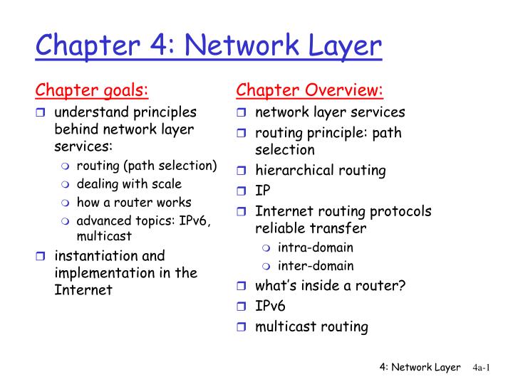
Chapter goals: understand principles behind network layer services: routing (path selection) dealing with scale how a router works advanced topics: IPv6, multicast instantiation and implementation in the Internet. Chapter Overview: network layer services routing principle: path selection

E N D
Chapter goals: understand principles behind network layer services: routing (path selection) dealing with scale how a router works advanced topics: IPv6, multicast instantiation and implementation in the Internet Chapter Overview: network layer services routing principle: path selection hierarchical routing IP Internet routing protocols reliable transfer intra-domain inter-domain what’s inside a router? IPv6 multicast routing Chapter 4: Network Layer 4: Network Layer
transport packet from sending to receiving hosts network layer protocols in every host, router three important functions: path determination: route taken by packets from source to dest. Routing algorithms switching: move packets from router’s input to appropriate router output call setup: some network architectures require router call setup along path before data flows network data link physical network data link physical network data link physical network data link physical network data link physical network data link physical network data link physical network data link physical application transport network data link physical application transport network data link physical Network layer functions 4: Network Layer
Q: What service model for “channel” transporting packets from sender to receiver? guaranteed bandwidth? preservation of inter-packet timing (no jitter)? loss-free delivery? in-order delivery? congestion feedback to sender? Network service model The most important abstraction provided by network layer: ? ? virtual circuit or datagram? ? service abstraction 4: Network Layer
call setup, teardown for each call before data can flow each packet carries VC identifier (not destination host OD) every router on source-destination path, s, maintains “state” for each passing connection transport-layer connection only involved two end systems link, router resources (bandwidth, buffers) may be allocated to VC to get circuit-like performance “source-to-destination path behaves much like telephone circuit” performance-wise network actions along source-to-destination path Virtual circuits 4: Network Layer
used to setup, maintain teardown VC used in ATM, frame-relay, X.25 not used in today’s Internet application transport network data link physical application transport network data link physical Virtual circuits: signaling protocols 6. Receive data 5. Data flow begins 4. Call connected 3. Accept call 1. Initiate call 2. incoming call 4: Network Layer
no call setup at network layer routers: no state about end-to-end connections no network-level concept of “connection” packets typically routed using destination host ID packets between same source-destination pair may take different paths application transport network data link physical application transport network data link physical Datagram networks: the Internet model 1. Send data 2. Receive data 4: Network Layer
Network layer service models: Guarantees ? Network Architecture Internet ATM ATM ATM ATM Service Model best effort CBR VBR ABR UBR Congestion feedback no (inferred via loss) no congestion no congestion yes no Bandwidth none constant rate guaranteed rate guaranteed minimum none Loss no yes yes no no Order no yes yes yes yes Timing no yes yes no no • Internet model being extented: Intserv, Diffserv • Chapter 6 4: Network Layer
Internet data exchange among computers “elastic” service, no strict timing req. “smart” end systems (computers) can adapt, perform control, error recovery simple inside network, complexity at “edge” many link types different characteristics uniform service difficult ATM evolved from telephony human conversation: strict timing, reliability requirements need for guaranteed service “dumb” end systems telephones complexity inside network Datagram or VC network: why? 4: Network Layer
Graph abstraction for routing algorithms: graph nodes are routers graph edges are physical links link cost: delay, $ cost, or congestion level 5 3 5 2 2 1 3 1 2 1 A D B E F C Routing protocol Routing Goal: determine “good” path (sequence of routers) thru network from source to dest. • “good” path: • typically means minimum cost path • other def’s possible 4: Network Layer
Routing Issues Key question: how are routing tables determined / updated? • who determines table entries? • what info used in determining table entries? • when do routing table entries change? • where is routing info stored? • how to control table size? • why are routing tables determined a particular way. What is the theoretical basis? Answer these and we are done! 4: Network Layer
Routing Issues… (more) • scalability: must be able to support large numbers of hosts, routers, networks • adapt to changes in topology or significant changes in traffic, quickly and efficiently • self-healing: little or not human intervention • route selection may depend on different criteria • performance: "choose route with smallest delay" • policy: "choose a route that doesn't cross a government network" (equivalently: "let no non-government traffic cross this network") 4: Network Layer
Classification of Routing Algorithms Centralized versus decentralized • centralized: central site computes and distributed routes (equivalently: information for computing routes known globally, each router makes same computation) • decentralized: each router sees only local information (itself and physically-connected neighbors) and computes routes on this basis • pros and cons? 4: Network Layer
Classification Static versus adaptive • static: routing tables change very slowly, often in response to human intervention • dynamic: routing tables change as network traffic or topology change • pros and cons ? Two basic approaches adopted in practice: • link-state routing: centralized, dynamic (periodically run) • distance vector: distributed, dynamic (in direct response to changes) 4: Network Layer
Global or decentralized information? Global: all routers have complete topology, link cost info “link state” algorithms Decentralized: router knows physically-connected neighbors, link costs to neighbors iterative process of computation, exchange of info with neighbors “distance vector” algorithms Static or dynamic? Static: routes change slowly over time Dynamic: routes change more quickly periodic update in response to link cost changes Routing Algorithm classification 4: Network Layer
Dijkstra’s algorithm net topology, link costs known to all nodes accomplished via “link state broadcast” all nodes have same info computes least cost paths from one node (‘source”) to all other nodes gives routing table for that node iterative: after k iterations, know least cost path to k dest.’s Not necessarily the fewest hops ! Notation: c(i,j): link cost from node i to j. cost infinite if not direct neighbors D(v): current value of cost of path from source to dest. V p(v): predecessor node along path from source to v, that is next v N: set of nodes whose least cost path definitively known A Link-State Routing Algorithm 4: Network Layer
Link-State Routing • flooding : router sends out information on all of its ports; its neighbors then send out information on all of their ports, etc…. Eventually every router ( no exceptions) receives a copy of the same information • Link State : each router periodically shares its knowledge of its neighborhood with all routers in the network 4: Network Layer
Link-state routing Link State Packet: When a router floods the network with information about its neighborhood, it is said to be advertising. The basis of this advertising is a short packet called a link state packet (LSP), usually containing 4 fields: • ID of advertiser, • ID of destination network affected, • the cost, • the ID of the neighbor router 4: Network Layer
Link-State Routing Algorithms How get information about neighbors ? Periodically sends them a short greeting packet • responds : assume ok and functioning well • no response: assume a change and alerts entire network in its next LSP • greeting pkt : small and use negligible resources ( unlike DV routing tables) Initialization Each router comes up and sends greeting packet to its neighbors; prepares a LSP and floods the network 4: Network Layer
Link State Database: • Every router receives every LSP and puts the information into a LS database • => every router builds the same database ( as all receive the same info) • To calculate the routing information, each router applies an algorithm( Dijkstra’s Algorithm) to calculate the shortest path between two points on a network of arcs and nodes • nodes = networks or routers • arcs = connections between router and network with costs applied only to the router==> network arc • network => router are always 0 cost 4: Network Layer
Dijsktra’s Algorithm 1 Initialization: 2 N = {A} 3 for all nodes v 4 if v adjacent to A 5 then D(v) = c(A,v) 6 else D(v) = infty 7 8 Loop 9 find w not in N such that D(w) is a minimum 10 add w to N 11 update D(v) for all v adjacent to w and not in N: 12 D(v) = min( D(v), D(w) + c(w,v) ) 13 /* new cost to v is either old cost to v or known 14 shortest path cost to w plus cost from w to v */ 15 until all nodes in N 4: Network Layer
Dijkstra’s Algorithm 1. Begins to build the shortest path tree by identifying its root - then attaching all nodes that can be reached from the root ( all the neighbors) -- nodes and arcs are temporary at this stage 2. Compares temporary arcs and identifies the one with lowest cumulative cost AND makes this arc and node a permanent connection 3. Examines the database and identifies every node that can be reached from its newly chosen node 4. Repeat steps 2 and 3 until every node in the network has become a permanent part of the tree -- the only permanent arcs will be those representing the shortest route to every node. • Routing Table Each router now uses the shortest path tree to construct its routing table - which are both different for each router 4: Network Layer
5 3 5 2 2 1 3 1 2 1 A D B E F C Dijkstra’s algorithm: example D(B),p(B) 2,A 2,A 2,A D(D),p(D) 1,A D(C),p(C) 5,A 4,D 3,E 3,E D(E),p(E) infinity 2,D Step 0 1 2 3 4 5 start N A AD ADE ADEB ADEBC ADEBCF D(F),p(F) infinity infinity 4,E 4,E 4,E 4: Network Layer
Algorithm complexity: n nodes each iteration: need to check all nodes, w, not in N n*(n+1)/2 comparisons: O(n**2) more efficient implementations possible: O(nlogn) Oscillations possible: e.g., link cost = amount of carried traffic A A A A D D D D B B B B C C C C 2+e 2+e 0 0 1 1 1+e 1+e 0 e 0 0 Dijkstra’s algorithm, discussion 1 1+e 0 2+e 0 0 0 0 e 0 1 1+e 1 1 e … recompute … recompute routing … recompute initially 4: Network Layer
Routing Protocol Requirements • Minimize routing table space: keep as small as possible – reduces overhead involved with sharing information • Minimize control messages • Robust : protect against corruption of tables; periodically run consistency checks, add sequence numbers • Use optimal paths 4: Network Layer
Distance Vector Routing Algorithm • Telephone network routing can take advantage of predictable traffic flow and a relatively small network core • Large packet networks are a very different environment • Links and routers are unreliable • Alternative paths may well be scarce • Traffic patterns change unpredictably within minutes 4: Network Layer
Routing algorithms Link state and distance vector algorithms both assume a router knows: • address of each neighbor • the cost of reaching each neighbor Both allow a router to find / discover global routing information, i.e. the next hop to reach every destination in the network by the shortest path by exchanging routing information with only its neighbors 4: Network Layer
Routing algorithms • Distance Vector algorithm: • A node tells its neighbors its distance to everyother node in the network • Link State algorithm: • A node tells every other node in the network its distance to neighbors • Both are distributed and suitable for large internetworks controlled by multiple administrative entities 4: Network Layer
Distance Vector Routing Algorithm • Assume each router knows the identity of every other router in the network – but not necessarily the shortest path to it. • Each router maintains a distance vector = list of < destination , cost > tuples , one per destination • Cost = sum o f the link costs on the shortest path to that destination • Initially , cost set to a value higher than expected cost of any route in the network ( hence to infinity ) 4: Network Layer
Distance Vector Routing Algorithm • Router periodically sends copy of its distance vector to all of its neighbors • When a distance vector is received, router determines whether its costs to any destination would decrease if it routed packets to that destination through that neighbor • With this asynchronous updating, eventually the routing tables converge • Info. Spread one hop at a time … method due to Bellman and Ford 4: Network Layer
iterative: continues until no nodes exchange info. self-terminating : no “signal” to stop asynchronous: nodes need not exchange info/iterate in lock step! distributed: each node communicates only with directly-attached neighbors Distance Table data structure each node has its own row for each possible destination column for each directly-attached neighbor to node example: in node X, for dest. Y via neighbor Z: distance from X to Y, via Z as next hop X = D (Y,Z) Z c(X,Z) + min {D (Y,w)} = w Distance Vector Routing Algorithm 4: Network Layer
wait for (change in local link cost of msg from neighbor) recompute distance table if least cost path to any dest has changed, notify neighbors Distance Vector Routing: overview Iterative, asynchronous: each local iteration caused by: • local link cost change • message from neighbor: its least cost path change from neighbor Distributed: • each node notifies neighbors only when its least cost path to any destination changes • neighbors then notify their neighbors if necessary Each node: 4: Network Layer
Distance Vector Routing • Each router shares its knowledge about the entire network by sending all of its collected knowledge to its neighbors. At the outset, this may be very sparse but it is all sent • Each router periodically sends its information only to those routers to which it has a direct connection - this info. is used by neighbors to update their own information • Roughly, every 30 seconds each router sends its information to its neighbors - whether or not network has changed since last exchange • recall Link State updates ~every 30 minutes • Distance Vector : each router periodically shares its knowledge of the entire network with each of its neighbors 4: Network Layer
Distance Vector Routing • Packet Cost: Both LS and DV are lowest cost algorithms • DV : cost refers to hop count • LS : cost refers a weighted value based on number of factors - security levels, traffic, state of the link,… • costs may well be different for the same 2 networks • In determining the route, cost of a hop is applied to each packet as it leaves a router and enters a network ( outbound cost) • costs are applied only to routers and not any other station on a network ( link from one router to next is a network NOT a point to point connection • costs are applied as packet leaves NOT as it enters a router • most networks are broadcast networks- when a packet enters a network, every station,including the router can pick it up - so don’t assign cost of going from network to router 4: Network Layer
Net:14 B Net:55 Net:14 Net:92 Net:78 A C F Net:66 Net:23 Net:08 D E 4: Network Layer
Routing Table • At startup , router’s knowledge is sparse - knows it is connected to some number of LANs and knows ID of each station. • In most systems, a station port ID and network ID share the same prefix router can discover to which nets it is connected by examining its own logical addresses (has as many such addresses as it has connected ports) • Routing Table : at least 3 pieces of info :Network ID, cost, ID of next router • Network ID = final destination of the packet • cost = # hops packet must take to get there • Next router = the router to which a packet is to be delivered on its way to destination • so for the diagram: initial table at A is • 14 1 - • 23 1 - • 78 1 - • only dest. at startup are those attached directly ==> blank in 3rd column • no multihop destinations identified , yet no next routers • These basic tables are sent out on network 4: Network Layer
Routing Table • When A receives info. table from B , it sees that B can get to nets 55 and 14; A knows B is its neighbor so if A adds 1 more hop to all costs shown in B table, the sum will be cost to A of getting to these other networks A old table combined A - new table Rec’d from B 4: Network Layer
1 DE() A B D A 1 14 5 B 7 8 5 C 6 9 4 D 4 11 2 B C 7 8 2 A Distance table: • per-node table recording cost to all other nodes via each of its neighbors • DE(A,B) gives currently computed minimum cost from E to A given that first node on path is B. • DE(A,B) = c(E,B) + min DB(A,*) • min DE(A,*) gives E's minimum cost to A • routing table derived from distance table • example: DE(A,B) = 14 (note: not 15!) • example: DE(C,D) = 4, DE(C,A) = 6 1 D E 2 4: Network Layer
Distance vector algorithm • based on Bellman-Ford algorithm • used in many routing protocols: Internet BGP, ISO IDRP, Novell IPX, original ARPAnet Algorithm (at node X): Initialization: for all adjacent nodes v: D(*,v) = infinity D(v,v) = c(X,v) send shortest path cost to each destination to neighbors Loop: execute distributed topology update algorithm forever This is the hardest component 4: Network Layer
Update Algorithm at Node X: 1. wait (until I see a link cost change to neighbor Y or until I receive an update from neighbor W) 2. if (c(X,Y) changes by delta) { /* change my cost to my neighbor Y */ change all column-Y entries in distance table by delta if this changes my least cost path to Z send update wrt Z, DX(Z,*) , to all neighbors } 3. if (update received from W wrt Z) { /* shortest path from W to some Z has changed */ DX(Z,W) = c(X,W) + DW(Z,*) } if this changes my least cost path to Z send update wrt Z, DX(Z,*) , to all neighbors } 4: Network Layer
cost to destination via E D () A B C D A 1 7 6 4 B 14 8 9 11 D 5 5 4 2 1 7 2 8 1 destination 2 A D B E C E E E D (C,D) D (A,D) D (A,B) B D D c(E,B) + min {D (A,w)} c(E,D) + min {D (A,w)} c(E,D) + min {D (C,w)} = = = w w w = = = 2+3 = 5 2+2 = 4 8+6 = 14 Distance Table: example loop! loop! 4: Network Layer
cost to destination via E D () A B C D A 1 7 6 4 B 14 8 9 11 D 5 5 4 2 destination Distance table gives routing table Outgoing link to use, cost A B C D A,1 D,5 D,4 D,4 destination Routing table Distance table 4: Network Layer
1 B C DE() A B D A 1 14 5 B 7 8 5 C 6 9 4 D 4 11 2 7 8 2 A 1 D E 2 Distance table: • per-node table recording cost to all other nodes via each of its neighbors • DE(A,B) gives currently computed minimum cost from E to A given that first node on path is B. • DE(A,B) = c(E,B) + min DB(A,*) • min DE(A,*) gives E's minimum cost to A • routing table derived from distance table • example: DE(A,B) = 14 (note: not 15!) • example: DE(C,D) = 4, DE(C,A) = 6 4: Network Layer
Iterative, asynchronous: each local iteration caused by: local link cost change message from neighbor: its least cost path change from neighbor Distributed: each node notifies neighbors only when its least cost path to any destination changes neighbors then notify their neighbors if necessary wait for (change in local link cost of msg from neighbor) recompute distance table if least cost path to any dest has changed, notify neighbors Distance Vector Routing: overview Each node: 4: Network Layer
Distance Vector Algorithm: At all nodes, X: 1 Initialization: 2 for all adjacent nodes v: 3 D (*,v) = infty /* the * operator means "for all rows" */ 4 D (v,v) = c(X,v) 5 for all destinations, y 6 send min D (y,w) to each neighbor /* w over all X's neighbors */ X X X w 4: Network Layer
Distance Vector Algorithm (cont.): 8 loop 9 wait (until I see a link cost change to neighbor V 10 or until I receive update from neighbor V) 11 12 if (c(X,V) changes by d) 13 /* change cost to all dest's via neighbor v by d */ 14 /* note: d could be positive or negative */ 15 for all destinations y: D (y,V) = D (y,V) + d 16 17 else if (update received from V wrt destination Y) 18 /* shortest path from V to some Y has changed */ 19 /* V has sent a new value for its min DV(Y,w) */ 20 /* call this received new value is "newval" */ 21 for the single destination y: D (Y,V) = c(X,V) + newval 22 23 if we have a new min D (Y,w)for any destination Y 24 send new value of min D (Y,w) to all neighbors 25 26 forever X X w X X w X w 4: Network Layer
2 1 7 Y Z X X c(X,Y) + min {D (Z,w)} c(X,Z) + min {D (Y,w)} D (Y,Z) D (Z,Y) = = w w = = 2+1 = 3 7+1 = 8 X Z Y Distance Vector Algorithm: example 4: Network Layer
2 1 1 X Z Y Distance Vector Algorithm: example 7 4: Network Layer
1 4 1 50 X Z Y Distance Vector: link cost changes Link cost changes: • node detects local link cost change • updates distance table (line 15) • if cost change in least cost path, notify neighbors (lines 23,24) algorithm terminates “good news travels fast” 4: Network Layer
60 4 1 50 X Z Y Distance Vector: link cost changes Link cost changes: • good news travels fast • bad news travels slow - “count to infinity” problem! Y Y Y algorithm continues on! 4: Network Layer
Topology Changes • suppose that A becomes aware that F has failed. How is this possible? • The mechanism used in RIP is the following: • Every router is supposed to send an update vector to its neighbors every 30 seconds. • If a node K has an entry in its routing table for network i with the next hop to router N, and if K receives no updates from N within 180 seconds, it marks the route invalid. • The assumption is made that either router N has crashed or that the network connecting K to N has become unstable. When K hears any neighbor has a valid route to i, the valid route replaces the invalid one. • The way in which a route is marked invalid is to set the value of the dist to the route to infinity. In practice, RIP uses a value of 16 to equal infinity. 4: Network Layer