Download
1 / 54
540 likes | 643 Views
NGS Part I RNA-Seq Short Reads Sequence Analysis Feb 29, 2012. Daniel Fernandez and Alejandro Quiroz dfernan@gmail.com aquiroz@hsph.harvard.edu. 1 st ACT (1 hour) Introduction INTERLUDE Chill Out Sessions with DJ Bowtie (10 min) 2 nd ACT (1 hour 50 min) Homework help Q4 and Q5.

E N D
NGS Part IRNA-SeqShort Reads Sequence AnalysisFeb 29, 2012 Daniel Fernandez and Alejandro Quiroz dfernan@gmail.com aquiroz@hsph.harvard.edu
1st ACT (1 hour) Introduction INTERLUDE Chill Out Sessions with DJ Bowtie (10 min) 2nd ACT (1 hour 50 min) Homework help Q4 and Q5.
Central Dogma of MB R E V E R S E E N G I N E E R I N G GENOME B I O L O G Y TRANSCRIPTOME
Reverse Engineering: We can use sequencing to find the genome state RNA-Seq Transcription Wang, Z Nature Reviews Genetics 2009
Reverse Engineering: Once sequenced the problem becomes computational Sequenced reads sequencer cells Library preparation Alignment read coverage genome
Overview of the session • We’ll cover the 3 main computational challenges of sequence analysis for counting applications: • Read mapping: Placing short reads in the genome • Reconstruction: Finding the regions that originated the reads • Quantification: • Assigning scores to regions • Finding regions that are differentially represented between two or more samples.
What software to use • If read quality is good (error rate < 1%) and there is a reference. BWA is a very good choice. • If read quality is not good or the reference is phylogenetically far (e.g. Wolf to dog) and you have a server with enough memory SHRiMP or BFAST should be a sensitive but relatively fast choice. What about RNA-Seq?
RNA-Seq read mapping is more complex than just sequencing 100s bp 10s kb RNA-Seq reads can be spliced, and spliced reads are most informative
Short read mapping software for RNA-Seq Exon-first alignments will map contiguous first at the expense of spliced hits
Microarrays Epigenomics RNA-Seq NGS alignments Comparative genomics IGV: Integrative Genomics Viewer • A desktop application • for the visualization and interactive exploration • of genomic data
Visualizing read alignments with IGV Long marks Medium marks Punctuate marks
Visualizing read alignments with IGV — RNASeq Gap between reads spanning exons
Visualizing read alignments with IGV — RNASeq close-up What are the gray reads? We will revisit later.
Overview of the session • The 3 main computational challenges of sequence analysis for counting applications: • Read mapping: Placing short reads in the genome • Reconstruction: Finding the regions that originate the reads • Quantification: • Assigning scores to regions • Finding regions that are differentially represented between two or more samples.
Scripture for RNA-Seq: Extending segmentation to discontiguous regions
The transcript reconstruction problem • Challenges: • Genes exist at many different expression levels, spanning several orders of magnitude. • Reads originate from both mature mRNA (exons) and immature mRNA (introns) and it can be problematic to distinguish between them. • Reads are short and genes can have many isoforms making it challenging to determine which isoform produced each read. 100s bp 10s kb There are two main approaches to this problem, first lets discuss Scripture’s
Scripture Overview Map reads Scan “discontiguous” windows Merge windows & build transcript graph Filter & report isoforms
Pros and cons of each approach • Transcript assembly methods are the obvious choice for organisms without a reference sequence. • Genome-guided approaches are ideal for annotating high-quality genomes and expanding the catalog of expressed transcripts and comparing transcriptomes of different cell types or conditions. • Hybrid approaches for lesser quality or transcriptomes that underwent major rearrangements, such as in cancer cell. • More than 1000 fold variability in expression leves makes assembly a harder problem for transcriptome assembly compared with regular genome assembly. • Genome guided methods are very sensitive to alignment artifacts.
Scripture was designed with annotation in mind. It reports all possible transcripts that are significantly expressed given the aligned data (Maximum sensitivity). • Cuffllinks was designed with quantification in mind. It limits reported isoforms to the minimal number that explains the data (Maximum precision). Differences between Cufflinks and Scripture
Differences between Cufflinks and Scripture - Example Annotation Scripture Cufflinks Alignments
Overview of the session • The 3 main computational challenges of sequence analysis for counting applications: • Read mapping: Placing short reads in the genome • Reconstruction: Finding the regions that originate the reads • Quantification: • Assigning scores to regions • Finding regions that are differentially represented between two or more samples.
Quantification Fragmentation of transcripts results in length bias: longer transcripts have higher counts Different experiments have different yields. Normalization is required for cross lane comparisons: Reads per kilobase of exonic sequence per million mapped reads (Mortazavi et al Nature methods 2008) This is all good when genes have one isoform.
Quantification with multiple isoforms How do we define the gene expression? How do we compute the expression of each isoform?
Computing gene expression Idea1: RPKM of the constitutive reads (Neuma, Alexa-Seq, Scripture)
Computing gene expression — isoform deconvolution If we knew the origin of the reads we could compute each isoform’s expression. The gene’s expression would be the sum of the expression of all its isoforms. E = RPKM1+ RPKM2 + RPKM3
Library construction improvements — Paired-end sequencing Adapted from the Helicos website
Paired ends increase isoformdeconvolution confidence • P1 originates from isoform 1 or 2 but not 3. • P2 and P3originate from isoform 1 Paired-end reads are easier to associate to isoforms P1 P3 P2 Isoform 1 Isoform 2 Isoform 3 Do paired-end reads also help identifying reads originating in isoform 3?
We can estimate the insert size distribution P1 P2 Get all single isoform reconstructions Splice and compute insert distance d1 d2 Estimate insert size empirical distribution
… and use it for probabilistic read assignment Isoform 1 Isoform 2 d2 d1 Isoform 3 d1 d2 P(d > di)
And improve quantification Katz et al Nature Methods 2008
Paired-end improve reconstructions Paired-end data complements the connectivity graph
And merge regions Single reads Paired reads
Or split regions Single reads Paired reads
Paired-end reads are now routine in Illumina and SOLiD sequencers. • Paired end alignment is supported by most short read aligners • Transcript quantification depends heavily in paired-end data • Transcript reconstruction is greatly improved when using paired-ends (work in progress) Summary
Several methods now exist to build strand sepecific RNA-Seq libraries. • Quantification methods support strand specific libraries. For example Scripture will compute expression on both strand if desired. Summary
Overview of the session • The 3 main computational challenges of sequence analysis for counting applications: • Read mapping: Placing short reads in the genome • Reconstruction: Finding the regions that originate the reads • Quantification: • Assigning scores to regions • Finding regions that are differentially represented between two or more samples.
Finding genes that have different expression between two or more conditions. • Find gene with isoforms expressed at different levels between two or more conditions. • Find differentially used slicing events • Find alternatively used transcription start sites • Find alternatively used 3’ UTRs The problem.
Differential gene expression using RNA-Seq • (Normalized) read counts Hybridization intensity • We observe the individual events.