Download
1 / 40
470 likes | 679 Views
Pattern Association. A pattern association learns associations between input patterns and output patterns. One of the most appealing characteristics of such a network is the fact that it can generate what it learns about one pattern to other similar input patterns.

E N D
Pattern Association • A pattern association learns associations between input patterns and output patterns. • One of the most appealing characteristics of such a network is the fact that it can generate what it learns about one pattern to other similar input patterns. • Pattern associations have been widely used in distributed memory modeling.
Pattern Association • The pattern association is one of the more basic two-layer networks. • Its architecture consists of two sets of units, the input units and the output units. • Each input unit connects to each output unit via weighted connections. • Connections are only allowed from input units to output units. • The effect of a unit uiin the input layer on a unit ujin the output layer is determined by the product of the activationaiof uiand the weight of the connection from ui to uj. The activation of a unit uj in the output layer is given by: SUM(wij * ai).
Pattern Association • A pattern association can be trained to respond with a certain output pattern when presented with an input pattern. • The connection weights can be adjusted in order to change the input/output behavior. • However, one of the most interesting properties of these models is their ability to self-modify and learn. • The learning rule is what specifies how a network changes it weights for a given input/output association. • The most commonly used learning rules with pattern associators are the Hebb rule and the Delta rule.
Each association is an input-output vector pair, s:t. • If each vector t is the same as the vector s with which it is associated, the net called auto-associative memory • If t’s are different from the s, the net is called hetero-associative memory
Training Algorithms For Pattern Association • Hebb Rule for Pattern Association • The simplest and most common method of determining the weights for an associative memory NN. • Can use pattern represented in binary or bipolar. • Similar algorithm with slight extension where finding the weights by outer products. • We want to consider examples in which the input to the net after training is a pattern that is similar to, but not the same as one of the training inputs.
Training Algorithms For Pattern Association • Hebb Rule for Pattern Association Step 0: Initialize all weights: wij = 0 (i= 1 … n; j = 1, …,m); Step 1: For each input training vector pair and target output pair, s:t, do steps 2-4 Step 2. Set activations for input units: xi = si (i = 1 to n). Step 3. Set activation for output unit: yj = tj (t= target) Step 4. Adjust the weights for wi,j(new) = wi,j(old) + xi yj (i= 1 … n; j = 1, …,m);
Outer products The weights found by using the Hebb rule with all weights initially 0) can also be described in terms of outer products of the input vector-output vector pairs. The outer products of two vectors s = (s1, …, si, …, sn) t = (t1, …, tj, … tm) Hebb Rule for Pattern Association
The outer products of two vectors s = (s1, …, si, …, sn) t = (t1, …, tj, … tm) ST = s1 : si : sn Hebb Rule for Pattern Association s1t1 …s1tj … s1tm : sit1 … sitj … sitm : snt1 … sntj … sntm = [t1, .., tj .. tm)
This is the weight matrix to store the association s:t found using Hebb rule To store a set of associations s(p) : t(p), p= 1, …, P, where s(p) = (si(p), …, si(p), …, sn(p)) and t(p) = (ti(p), …, ti(p), …, tm(p)) the weight matrix W = {wij} is given by wij = si(p) ti(p) or in general W = sT(p) t (p) Hebb Rule for Pattern Association P P p=1 p=1
Using Hebb’s Law we can express the adjustment applied to the weight wij at iteration p in the following form: • As a special case, we can represent Hebb’s Law as follows: where is the learning rate parameter. This equation is referred to as the activity product rule.
Hebbian learning implies that weights can only increase. To resolve this problem, we might impose a limit on the growth of synaptic weights. It can be done by introducing a non-linear forgetting factor into Hebb’s Law: where is the forgetting factor. Forgetting factor usually falls in the interval between 0 and 1, typically between 0.01 and 0.1, to allow only a little “forgetting” while limiting the weight growth.
Hebbian learning algorithm Step 1: Initialisation. Set initial synaptic weights and thresholds to small random values, say in an interval [0, 1]. Step 2: Activation. Compute the neuron output at iteration p where n is the number of neuron inputs, and j is the threshold value of neuron j.
Step 3:Learning. Update the weights in the network: where wij(p) is the weight correction at iteration p. The weight correction is determined by the generalised activity product rule: Step 4: Iteration. Increase iteration p by one, go back to Step 2.
Hebbian learning example To illustrate Hebbian learning, consider a fully connected feedforward network with a single layer of five computation neurons. Each neuron is represented by a McCulloch and Pitts model with the sign activation function. The network is trained on the following set of input vectors:
O u t p u t l a y e r O u t p u t l a y e r 2 4 5 2 4 5 1 3 1 3 é é ù 0 0 0 0 0 0 0 0 0 0 1 1 ê ê ú 0 0 2.0204 0 1 0 0 1 0 2.0204 2 2 ê ê ú I n p u t l a y e r ê ê ú 1.0200 0 0 0 0 1 0 0 0 0 3 3 ê ê ú 0 0.9996 0 0 0 0 1 0 0 0 4 4 ê ú ê ê ê ú 0 0 2.0204 0 1 0 0 1 0 2.0204 5 5 ë ë û ( b ). Initial and final weight matrices ù ú ú I n p u t l a y e r ú ú ú ú û
A test input vector, or probe, is defined as • When this probe is presented to the network, we obtain:
P2 P1 P3 Pt Example 2 Consider the three prototype patterns shown. i. Use the Hebb rule to design a perceptron network that will recognize these three patterns • Find the respond of the network • To the pattern Pt. • Is the response correct?
P2 P1 P3 Pt t1 = t3 = P2= Pt= P1 = P3 = t2 = --1 1 -1 -1 1 -1 1 1 1 -1 -1 -1 -1 1 1 1 -1 1 1 -1 1 1 - Example 2 Convert patterns to vectors
-3 -1 -1 -1 1 3 -1 -1 -1 -1 1 -1 1 -1 Example 2 Determine the weight matrix using the Hebb rule 1 -1 1 1 1 1 -1 1 -1 -1 -1 1 -1 -1 1 -1 1 -1 -3 -1 -1 -1 1 3 -1 -1 W = TPT = = Find the respond of the network To the pattern Pt. A = hardlims(Wpt) = hardlims -2 -2 = hardlims = P1
The Hopfield Network • Neural networks were designed on analogy with the brain. The brain’s memory, however, works by association. For example, we can recognise a familiar face even in an unfamiliar environment within 100-200 ms. We can also recall a complete sensory experience, including sounds and scenes, when we hear only a few bars of music. The brain routinely associates one thing with another.
Multilayer neural networks trained with the back-propagation algorithm are used for pattern recognition problems. However, to emulate the human memory’s associative characteristics we need a different type of network: a recurrent neural network. • A recurrent neural network has feedback loops from its outputs to its inputs. The presence of such loops has a profound impact on the learning capability of the network.
The stability of recurrent networks intrigued several researchers in the 1960s and 1970s. However, none was able to predict which network would be stable, and some researchers were pessimistic about finding a solution at all. The problem was solved only in 1982, when John Hopfield formulated the physical principle of storing information in a dynamically stable network.
The Hopfield network uses McCulloch and Pitts neurons with the sign activation function as its computing element:
The current state of the Hopfield network is determined by the current outputs of all neurons, y1, y2, . . ., yn. Thus, for a single-layer n-neuron network, the state can be defined by the state vector as:
In the Hopfield network, synaptic weights between neurons are usually represented in matrix form as follows: where M is the number of states to be memorised by the network, Ym is the n-dimensional binary vector, I is nn identity matrix, and superscript T denotes a matrix transposition.
The stable state-vertex is determined by the weight matrix W, the current input vector X, and the threshold matrix . If the input vector is partially incorrect or incomplete, the initial state will converge into the stable state-vertex after a few iterations. • Suppose, for instance, that our network is required to memorise two opposite states, (1, 1, 1) and (1, 1, 1). Thus, or where Y1 and Y2 are the three-dimensional vectors.
The 3 3 identity matrix I is • Thus, we can now determine the weight matrix as follows: • Next, the network is tested by the sequence of input vectors, X1 and X2, which are equal to the output (or target) vectors Y1 and Y2, respectively.
First, we activate the Hopfield network by applying the input vector X. Then, we calculate the actual output vector Y, and finally, we compare the result with the initial input vector X.
The remaining six states are all unstable. However, stable states (also called fundamental memories) are capable of attracting states that are close to them. • The fundamental memory (1, 1, 1) attracts unstable states (1, 1, 1), (1, 1, 1) and (1, 1, 1). Each of these unstable states represents a single error, compared to the fundamental memory (1, 1, 1). • The fundamental memory (1, 1, 1) attracts unstable states (1, 1, 1), (1, 1, 1) and (1, 1, 1). • Thus, the Hopfield network can act as an error correction network.
Storage capacity of the Hopfield network • Storage capacity is or the largest number of fundamental memories that can be stored and retrieved correctly. • The maximum number of fundamental memories Mmax that can be stored in the n-neuron recurrent network is limited by
Bidirectional associative memory (BAM) • The Hopfield network represents an autoassociative type of memory it can retrieve a corrupted or incomplete memory but cannot associate this memory with another different memory. • Human memory is essentially associative. One thing may remind us of another, and that of another, and so on. We use a chain of mental associations to recover a lost memory. If we forget where we left an umbrella, we try to recall where we last had it, what we were doing, and who we were talking to. We attempt to establish a chain of associations, and thereby to restore a lost memory.
To associate one memory with another, we need a recurrent neural network capable of accepting an input pattern on one set of neurons and producing a related, but different, output pattern on another set of neurons. • Bidirectional associative memory(BAM), first proposed by Bart Kosko, is a heteroassociative network. It associates patterns from one set, set A, to patterns from another set, set B, and vice versa. Like a Hopfield network, the BAM can generalise and also produce correct outputs despite corrupted or incomplete inputs.
The basic idea behind the BAM is to store pattern pairs so that when n-dimensional vector X from set A is presented as input, the BAM recalls m-dimensional vector Y from set B, but when Y is presented as input, the BAM recalls X.
To develop the BAM, we need to create a correlation matrix for each pattern pair we want to store. The correlation matrix is the matrix product of the input vector X, and the transpose of the output vector YT. The BAM weight matrix is the sum of all correlation matrices, that is, where M is the number of pattern pairs to be stored in the BAM.
Stability and storage capacity of the BAM • The BAM is unconditionally stable. This means that any set of associations can be learned without risk of instability. • The maximum number of associations to be stored in the BAM should not exceed the number of neurons in the smaller layer. • The more serious problem with the BAM is incorrect convergence. The BAM may not always produce the closest association. In fact, a stable association may be only slightly related to the initial input vector.