Download
1 / 49
540 likes | 1.01k Views
Association Rules and Frequent Pattern Analysis. Contents of this Chapter 5.1 Introduction 5.2 Basic Association Rules 5.3 Constraint-Based Association Mining 5.4 Multilevel Association Rules. Introduction. Motivation {butter, bread, milk, sugar}

E N D
Association Rules and Frequent Pattern Analysis • Contents of this Chapter • 5.1 Introduction • 5.2 Basic Association Rules • 5.3 Constraint-Based Association Mining • 5.4 Multilevel Association Rules SFU, CMPT 741, Fall 2009, Martin Ester
Introduction • Motivation • {butter, bread, milk, sugar} • {butter, flour, milk, sugar} • {butter, eggs, milk, salt} DB of Sales Transactions • {eggs} • {butter, flour, milk, salt, sugar} • Market basket analysis • Which products are frequently purchased together? • Applications • Improvement of store layouts • Cross marketing • Attached mailings/add-on sales SFU, CMPT 741, Fall 2009, Martin Ester
Introduction Association Rules • Rule form • “Body ® Head [support, confidence]” • Examples buy(X, “diapers”) ® buy(X, “beer”) [0.5%, 60%] major(X, “cs”) ^ takes(X, “db”) ® grade(X, “A”) [1%, 75%] 98% of all customers that buy car tires and assecories, bring their cars for service Buy both Buy beer Buy diapers SFU, CMPT 741, Fall 2009, Martin Ester
Introduction Frequent Patterns • Basic assumption Frequent patterns are more interesting than infrequent ones • Major challenge Efficiently finding (all) frequent patterns • Types of frequent patterns • Frequent item sets (boolean attributes) • Generalized frequent item sets (boolean attributes with concept hierarchies) • Quantitative frequent sets (numerical attributes) • Frequent sequences (sequence data) Mining biological data • Frequent subgraphs . . . SFU, CMPT 741, Fall 2009, Martin Ester
Basic Association Rules • Definitions [Agrawal & Srikant 1994] • Items I = {i1, ..., im} a set of literals • Item set X: set of items XI • DatabaseD: set of transactionsTi where TiI • TcontainsX: XT • Items in transactions or item sets are sorted in lexicographic order: • Item set X = (x1, x2, ..., xk ), where x1x2 ... xk • Length of item set: number of elements of item set • k-itemset: item set of length k SFU, CMPT 741, Fall 2009, Martin Ester
Basic Association Rules • Definitions • Support of item set X in D: percentage of transactions in D containing X • Frequent item set X in D: item set X with support³ minsup • Association rule: implication of the form XY, • where XI, YI and XY = SFU, CMPT 741, Fall 2009, Martin Ester
Basic Association Rules • Definitions • Support s of association rule X Y in D: • support of XY in D • Confidence c of association rule X Y in D: • percentage of transactions containing Y in the subset of all transactions in D that contain X • Task: discover all association rules that have support ³ minsup and confidence ³minconf in D SFU, CMPT 741, Fall 2009, Martin Ester
Basic Association Rules • Example minsup = 50%, minconf = 50% • Support • (A): 75%, (B), (C): 50%, (D), (E), (F): 25%, • (A, C): 50%, (A, B), (A, D), (B, C), (B, E), (B, F), (E, F): 25% • Association rules • A C (support = 50%, confidence = 66.6%) • C A (support = 50%, confidence= 100%) SFU, CMPT 741, Fall 2009, Martin Ester
Basic Association Rules • Two-Step Approach • 1. Determine the frequent item sets in the database • „Naive“ algorithm: • count the frequencies of all k-itemsets I • inefficient, sincesuch item sets • 2. Generate the association rules from the frequent item sets • Item set X frequent and AX • A (X-A) satisfies minimum support constraint • confidence has to be checked SFU, CMPT 741, Fall 2009, Martin Ester
Computation of the Frequent Item Sets • Basics • Monotony property • Each subset of a frequent item set is also frequent • If subset is not frequent, then superset cannot be frequent • Method • Determine first the frequent 1-item sets, then the frequent 2-item sets, . . . • To determine the frequent k+1-item sets: • consider only the k+1-item sets for which all k-subsets are frequent • Calculation of support: • one DB scan counting the support for all „relevant“ item sets SFU, CMPT 741, Fall 2009, Martin Ester
Computation of the Frequent Item Sets • Ck: set of candidate item sets of length kLk: set of all frequent item sets of length k • Apriori(D, minsup) • L1 := {frequent 1-itemsets inD}; • k := 2; • whileLk-1¹do Ck := AprioriCandidateGeneration(Lk- 1); for eachtransaction TDdo CT := subset(Ck, T); // all candidates fromCk, that are // contained in transactionT; for eachcandidatecCT do c.count++; Lk := {cCk | (c.count / |D|) minsup}; k++; • returnkLk; SFU, CMPT 741, Fall 2009, Martin Ester
Computation of the Frequent Item Sets • Candidate Generation • Requirements for set Ck of candidate itemsets • Superset of Lk • Significantly smaller than set of all k-subsets of I • Step 1: Join • Frequent k-1-item sets p and q • p and q are joined, if they agree in their first k-2 items • pÎ Lk-1 (1, 2, 3) • (1, 2, 3, 4) Î Ck • qÎ Lk-1 (1, 2, 4) SFU, CMPT 741, Fall 2009, Martin Ester
Computation of the Frequent Item Sets • Candidate Generation • Step 2: Pruning • Remove all elements from Ck having a k-1-subset not contained in Lk-1 • Example • L3 = {(1 2 3), (1 2 4), (1 3 4), (1 3 5), (2 3 4)} • After join step: C4 = {(1 2 3 4), (1 3 4 5)} • In pruning step: remove (1 3 4 5) • C4 = {(1 2 3 4)} SFU, CMPT 741, Fall 2009, Martin Ester
minsup = 2 C1 L1 Scan D L2 C2 C2 Scan D C3 L3 Scan D Computation of the Frequent Item Sets • Example SFU, CMPT 741, Fall 2009, Martin Ester
Computation of the Frequent Item Sets • Efficient Support for the Subset Function • Subset(Ck,T)all candidatesfromCk, that are contained in transactionT • Problems • Very large number of candidateitemsets • One transaction may contain many candidates • Hash tree as data structure for Ck • Leaf node records list of item sets(with frequencies) • Inner node contains hash table (apply hash function to d-th elements) each hash bucket at level d references son node at level d+1 • Root has level 1 SFU, CMPT 741, Fall 2009, Martin Ester
Computation of the Frequent Item Sets • Example h(K) = K mod 3 for 3-item sets 0 1 2 0 1 2 0 1 2 0 1 2 0 1 2 0 1 2 (2 5 6) (3 6 7) (3 5 7) (7 9 12) (1 4 11) (7 8 9) (2 3 8) (2 5 7) (3 5 11) (1 6 11) (1 7 9) (1 11 12) (5 6 7) (5 8 11) (3 7 11) (3 4 15) (2 4 6) (2 4 7) (3 4 11) (2 7 9) (5 7 10) (3 4 8) SFU, CMPT 741, Fall 2009, Martin Ester
Computation of the Frequent Item Sets • Hash Tree • Finding an item set • Start from the root • At level d: apply hash function h to the d-th element of the item set • Inserting an item set • Search the corresponding leaf node and insert new item set • In case of overflow: • Convert leaf node into inner node and create all its son nodes (new leaves) • Distribute all entries over the new leaf nodes according to hash function h SFU, CMPT 741, Fall 2009, Martin Ester
Computation of the Frequent Item Sets • Hash Tree • Find all candidates contained in T = (t1t2 ... tm) • At root • Determine hash values h(ti) for each item ti in T • Continue search in all corresponding son nodes • At inner node of level d • Assumption: inner node has been reached by hashing ti • Determine hash values and continue search for all items tk in T with k > i • At leaf node • For each item set X in this node, test whether XT SFU, CMPT 741, Fall 2009, Martin Ester
Leaf node to be tested Pruned subtree Computation of the Frequent Item Sets • Example Transaction (1, 3, 7, 9, 12) h(K) = K mod 3 0 1 2 3, 9, 12 1, 7 0 1 2 0 1 2 0 1 2 9, 12 7 3, 9, 12 7 0 1 2 0 1 2 (2 5 6) (3 6 7) (3 5 7) (7 9 12) (1 4 11) (7 8 9) (2 3 8) (2 5 7) (3 5 11) (1 6 11) (1 7 9) (1 11 12) (5 6 7) (5 8 11) 9, 12 (3 7 11) (3 4 15) (2 4 6) (2 4 7) (3 4 11) (2 7 9) (5 7 10) (3 4 8) SFU, CMPT 741, Fall 2009, Martin Ester
Computation of the Frequent Item Sets • Methods of Efficency Improvement • Support counting using a hash table [Park, Chen & Yu 1995] • Hash table instead of hash tree, support counters for hash buckets • k-item set with corresponding bucket counter < minsup cannot be frequent more efficient access to candidates but inaccurate counts • Reduction of transactions [Agrawal & Srikant 1994] • Transactions that do not contain any frequent k-item set are irrelevant • Remove such transactions for future phases more efficient DB scan, but additional writing of DB SFU, CMPT 741, Fall 2009, Martin Ester
Computation of the Frequent Item Sets • Methods of Efficency Improvement • Partitioning of the database [Savasere, Omiecinski & Navathe 1995] • Item set is only frequent if frequent in at least one partition • Form memory-resident partitions of the database • more efficient on partitions, but expensive combination of intermediate results • Sampling [Toivonen 1996] • Apply algorithm to sample to find frequent item sets • Count support of these frequent item sets in the whole database • Determine further candidates and support counting on the whole database SFU, CMPT 741, Fall 2009, Martin Ester
Computation of the Association Rules • Method • Frequent item set X • For each (frequent!) subset A of X, form the rule A (X-A) • Compute confidence of the rule A (X-A) • Discard rules that do not have minimum confidence • Store frequent item sets with their supports in a hash table • no DB accesses (no disk I/O) SFU, CMPT 741, Fall 2009, Martin Ester
Interestingness of Association Rules • Motivation • Application • Data about the behavior of students at a school with 5000 students • Example • Item sets with support: • 60% of the students play soccer, 75% of the students eat candy bars • 40% of the students play soccer and eat candy bars • Association rules: • „play soccer“ „eat candy bars“, confidence = 67% • TRUE „eat candy bars“, confidence = 75% • „play soccer“ and „eat candy bars“ are negatively correlated SFU, CMPT 741, Fall 2009, Martin Ester
Interestingness of Association Rules • Method • Filter out misleading association rules • Requirement for rule AB • for a constant d > 0 • Interestingness measure for rule AB • The larger this measure, the more interesting the discovered relationship between A and B. SFU, CMPT 741, Fall 2009, Martin Ester
Presentation of Association Rules DBMiner System [Han et al. 1996] SFU, CMPT 459 / 741, 06-3, Martin Ester
Presentation of Association Rules • Condition Consequent DBMiner System [Han et al. 1996] SFU, CMPT 459 / 741, 06-3, Martin Ester
Presentation of Association Rules DBMiner System [Han et al. 1996] SFU, CMPT 459 / 741, 06-3, Martin Ester
Constraint-Based Association Mining • Motivation • Too many frequent item sets • mining is inefficient • Too many association rules • hard to evaluate • Constraints may be known apriori „only association rules on product A but not on product B“ „only association rules with total price > 100“Constraints on the frequent item sets SFU, CMPT 741, Fall 2009, Martin Ester
Constraint-Based Association Mining • Types of Constraints [Ng, Lakshmanan, Han & Pang 1998] • Domain Constraints • S v, { , , , , , }, e.g. S.price < 100 • v S, {, },e.g. snacks S.type • V S or S V, { , , , , }, e.g.{snacks, wines} S.type • Aggregation Constraints agg(S) v where • agg {min, max, sum, count, avg} • { , , , , , }e.g. count(S1.type) 1, avg(S2.price) > 100 SFU, CMPT 741, Fall 2009, Martin Ester
Constraint-Based Association Mining • Application of the Constraints • When determining the association rules • Solves the evaluation problem • But not the efficiency problem • When determining the frequent item sets • Can also solve the efficiency problem • Challenge for candidate generation: Which candidate item sets can be pruned using the constraints? SFU, CMPT 741, Fall 2009, Martin Ester
Constraint-Based Association Mining • Anti-Monotonicity • Definition • If an item set S violates an anti-monotone constraint C, then all supersets of S violate this constraint. • Examples • sum(S.price) v is anti-monotone • sum(S. price) v is not anti-monotone • sum(S. price) = v is partly anti-monotone • Application Push anti-monotone constraintsinto candidate generation SFU, CMPT 741, Fall 2009, Martin Ester
Constraint-Based Association Mining S v, { , , } v S S V S V S V min(S) v min(S) v min(S) v max(S) v max(S) v max(S) v count(S) v count(S) v count(S) v sum(S) v sum(S) v sum(S) v avg(S) v, { , , } (frequent constraint) yes no no yes partly no yes partly yes no partly yes no partly yes no partly no (yes) Types of Constraints anti-monotone? SFU, CMPT 741, Fall 2009, Martin Ester
Multilevel Association Rules • Motivation • In many applications: taxonomies of items (is-a hierarchies) • Search for association rules at the leaf level: support may be too low • Search for association rules at the top level: patterns may be common sense • search for association rules at multiple (all) levels of the taxonomy Clothes Shoes Outerwear Underwear Walking-Shoes Hiking boots Jackets Trousers SFU, CMPT 741, Fall 2009, Martin Ester
Multilevel Association Rules • Motivation • Example • Anorak Hiking boots • Windcheater Hiking boots • Jacket Hiking boots Support > minsup • Properties • Support of „Jacket Hiking boots “ may be different from support of „ Anorak Hiking boots“ + support of „Windcheater Hiking boots“ • If „Jacket Hiking boots“ has minimum support, • then also „Outerwear Hiking boots“ Support < minsup SFU, CMPT 741, Fall 2009, Martin Ester
Multilevel Association Rules • Definitions[Srikant & Agrawal 1995] • I = {i1, ..., im} a set of literals („Items“) • H a directed acyclic graph over I • Edge in H from i to j : • i is a generalization of j, • i is called father or direct predecessor of j, • j is a son or direct sucessor of i. • is predecessor of x (xsuccessor of ) w.r.t. H: • there is a path from to x in H • Set of items is predecessor of set of items Z: • at least one item in predecessor of an item in Z SFU, CMPT 741, Fall 2009, Martin Ester
Multilevel Association Rules • Definitions • D is a set of transactions T, where TI • Typically: • Transactions T contain only elements from the leaves of graph H • Transaction Tsupportsitem iI: • iT or i is predecessor of an item jT • T supports set XI of items: • T supports each item in X • Support of set XI of items in D : • Percentage of transactions in D supporting X SFU, CMPT 741, Fall 2009, Martin Ester
Multilevel Association Rules • Definitions • Multilevel association rule: • XY where XI, YI, XY = • and no item in Y is predecessor w.r.t. H of an item in X • Support s of a multilevel association rule X Y in D : • Support of set XY in D • Confidence c of a multilevel association rule X Y in D: • Percentage of transactions containing Y in the subset of all transactions in D that contain X SFU, CMPT 741, Fall 2009, Martin Ester
Multilevel Association Rules • Example • Support of {Jackets}: 4 of 6 = 67% • Support of {Jackets, Hiking boots}: 2 of 6 = 33% • „Hiking-boots Jackets“: Support 33%, Confidence 100% • „ Jackets Hiking-boots“: Support 33%, Confidence 50% SFU, CMPT 741, Fall 2009, Martin Ester
Determining the Frequent Item Sets • Idea • Extend database transactions by all predecessors of items contained in that transaction • Method • Insert each item in transaction T together with all its predessors w.r.t. H into new transaction T’ • Do not insert duplicates • Then: • Determine frequent item sets for basic association rules (e.g. Apriori algorithm) • Basic algorithm for multilevel association rules SFU, CMPT 741, Fall 2009, Martin Ester
Determining the Frequent Item Sets • Optimizations of the Basic Algorithm • Materialization of Predecessors • Additional data structure H • Item ®list of all its predecessors • More efficient access to the predecessors • Filtering the predecessors to be added • Add only those predecessors that occur in an element of candidate set Ck • Example: Ck = {{Clothes, Shoes}} • replace „JacketXY“ by „ Clothes“ SFU, CMPT 741, Fall 2009, Martin Ester
Determining the Frequent Item Sets • Optimizations of the Basic Algorithm • Discard redundant item sets • Let X an k-item set, i an item and a predecessor of i. • Support of X- { } = support of X • X can be discarded during candidate generation • Do not need to count support of k-item set that contains item i and predecessor of i Algorithm Cumulate SFU, CMPT 741, Fall 2009, Martin Ester
Determining the Frequent Item Sets • Stratification • Alternative to the basic algorithm (Apriori-algorithm) • Stratification = form layers in the candidate sets • Property • Itemset is infrequent and is predecessor of X: • X is infrequent • Method • Do not count all k-itemsets at the same time • Count support first for the more general itemsets and count more special item sets only if necessary SFU, CMPT 741, Fall 2009, Martin Ester
Determining the Frequent Item Sets • Stratification • Example • Ck = {{Clothes Shoes}, {Outerwear Shoes}, {Jackets Shoes} } • Count support first for {Clothes Shoes} • Count support for Support für {Outerwear Shoes} only if {Clothes Shoes} is frequent • Notations • Depth of an item set: For itemsets X in candidate set Ck without direct predecessor in Ck: Depth(X) = 0. For all other item sets X in Ck: Depth(X) = max{Depth() | ÎCk is direct predecessor of X} + 1. • (Ckn): Set of item sets from Ck with depth n, 0 £n£ maximal depth t SFU, CMPT 741, Fall 2009, Martin Ester
Determining the Frequent Item Sets • Stratification • Algorithm Stratify • Count item sets in Ck0 • Remove all sucessors of infrequent elements of (Ck0) • Count support for remaining elements of (Ck1) • . . . • Trade-off between number of item sets for which the support is counted (memory requirements) and the number of database scans (I/O cost) • if |Ckn| small, then count candidates of depths (n, n+1, ..., t) at the same time SFU, CMPT 741, Fall 2009, Martin Ester
Determining the Frequent Item Sets • Stratification • Problems of Stratify • If many item sets of small depth are frequent: • Can discard only few item sets of larger depths • Improvements of Stratify • Estimate support of all item sets in Ck using a sample • Ck’: all item sets which have estimated support exceeding minimum support • Determine actual support of all itemsets in Ck’ in one database scan • Remove all successors of infrequent elements of Ck’ from Ck’’, • Ck’’ = Ck-Ck’ • Determine support for the remaining elements of Ck’’ in a second database scan SFU, CMPT 741, Fall 2009, Martin Ester
Interestingness of Multilevel Association Rules • Notations • is predecessor of : • Item set is predecessor of item set X and/or item set is predecessor • of set Y • direct predecessor of in a set of rules: • ispredecessor of , and there is no rule , such that predecessor of and predecessor of • Multilevel association rule is R-interesting: • Has no direct predecessors or • Actual support (confidence) > R times the expected support (confidence) • And the direct predecessor is also R-interesting. SFU, CMPT 741, Fall 2009, Martin Ester
Interestingness of Multilevel Association Rules • Example • Rule-No Rule Support R-interesting? • 1 Clothes Shoes 10 yes, no predecessor • 2 Outerwear Shoes 9 yes, support » R * expected support (w.r.t. rule 1) • 3 Jackets Shoes 4 no, support < R * expected support (w.r.t. rule 2) R = 2 SFU, CMPT 741, Fall 2009, Martin Ester
Outerwear Support = 10 % Jackets Support = 6 % Trousers Support = 4 % Multilevel Association Rules • Choice of minsup • Fix support • Variable support minsup = 5 % minsup = 5 % Outerwear Support = 10 % minsup = 5 % Jackets Support = 6 % Trousers Support = 4 % minsup = 3 % SFU, CMPT 741, Fall 2009, Martin Ester
Multilevel Association Rules • Discussion • Fix support • Same minsup value for all levels of the item taxonomy • + Efficiency: pruning successors of infrequent itemsets • - Reduced effectiveness minsup too high no low-level associations minsup too low too many high-level associations • Variable support • Different minsup values for different levels of the item taxonomy • + Good effectiveness • Find association rules at appropriate support level • - Inefficient: no pruning of successors of infrequent itemsets SFU, CMPT 741, Fall 2009, Martin Ester