Download
1 / 14
140 likes | 142 Views
This document discusses the challenges and conclusions of using CALICE as a high granularity calorimeter system for particle flow measurement in multi-jet final states at the ILC. It provides an overview of the different flavors/technologies used, the characteristics of the system, and the alignment and noise considerations. It also explores the potential use of CALICE in the ATLAS and LHC experiments.

E N D
CALICE as timing detector Dirk Zerwas LAL Orsay April 5, 2016 • CALICE • Challenges • Conclusions
CALICE • CALICE origin: A high granularity calorimeter system optimized for the particle flow measurement of multi-jet final states at the ILC running, with center-of-mass energy between 90GeV and ~1TeV • Electromagnetic and hadroniccalorimeters • Differentflavors/technologies: • SiW ECAL • Scintillator ECAL • Semi-digital HCAL • Analog HCAL • Characteristics: • Compact and granular: • EM thickness 20cm (R=1.8 to 2m) • up to 30 layers in depth • Lateral RO cell size 5.5mm x 5.5mm • High Granularity: 50M channels • Electronics/beam structure: • Bunch trains: 5Hz with 1ms length • Power-pulsedelectronics • 550ns betweenbunches • Triggerless running
Alveola (trapezoidal structure) • Attached to HCAL • Absorber: tungsten (structure) (+carbon structure) • Detector modules (SLABS) are placed in drawers • FE electronics on-detector • Digital RO electronics at the end in 3cm (!)
SLABs are subdividedintoASUs • ASUsconnected via kapton foils • Up to 10 ASUs per Slab • Interconnectionwithkapton foils (soldered) • Active cellscoverinterconnection to minimizedeadzones (0.5mm+0.5mm on 90mm) • ASU: • 18cm x 18cm • 4 Wafers (9cm x 9cm) glued to PCB • 5.5mm x 5.5mm cells • 1024 channels • « Only » 16 chips with 64 channelseachon a PCB
Alignment is essential: • PCB = 180.3 mm maximum • Wafer = 90 mm • As well as planarity/height of PCB+Chips • BGA • Wirebonded chips
Calorimeter Noise • Calorimetercell noise: • Large cells in the LArInnerWheel (>2.5): 0.1 x 0.1 • Only 2 samplings: • Significantincrease of noise for eta>2.5 • Rough equivalence: • 5mm • 0.008 at η=2.5 R=600mm • 0.017 at η=3.2 R=290mm • 0.037 at η=4.0 R=130mm • 0.096 at η=5.0 R=50mm Reference: Scoping document https://cds.cern.ch/record/2055248/files/LHCC-G-166.pdf
Arrival time spread for different BX schemes: • Assumption: z position isknown • Crabkissingreduces the time spread of the hard scatter (today200ps) to (greaterthan) 50ps • Efficiency hard scatter versus pileup: • Reduction of pileup as function of the timing resolution • pTjets>20GeV • Alg1: highestpTparticle • Alg2: time fraction • Gain of factor 10 possible (depends on working point)
CALICE in ATLAS • HGTD: • Replaces MBTS • Reducepileup in phase-2 • timing to determine vertex • Order 50ps • HGTD position: • z=3500mm • 2.5<η<5 • 600mm>r>48mm • HGTD envelope: • Δz=60mm • 4 layers in depth • Cell size order 5.5mm x 5.5mm • Order 300k cells • HGTD timing detector: • No abs • HGTD preshower detector: • 3 absorbers • Absorbers in front of LArg IW only: 2.5<η<3.2, 600mm>r>175mm
« Preshower » 53mm « Timing » 43mm
HGTD LHC based on CALICE • LHC • measurement: t and E • 4 layers in depth (z) • Granularity: 5.5mm x 5.5mm • option: mix withothergranularities • Same basic structure • Timing detector • Preshower detector (Tungsten) • Weakerconstraints: • 4 layers in 6cm ~1.5cm per layer • Harsherconstraints: • Cooling of sensors -20deg • RadHardness of FE electronics • RadHardness of Glue (done: 10^13, furtherforeseen in 2016) • Time measurement (order 50ps) • Shorterpeaking time • 40MHz • ILC • Measurement: E (and t) • 30 layers • Absorber: tungsten • 30 layers in 18cm ~0.6cm per layer • Cooling of electronics (passive) • Zero suppression/Power pulsing • 5Hz 1ms bunchtrain
Sketch of an Endcapimplementation Down to η=5 ischallenging Needsopeningmechanics R=110mm, η=4.1 Preserve basic CALICE structure R=600mm, η =2.4 • Slabs CALICE-like: • 2ASUs • 3ASUs • Alternative: • Single PCB • Pro: less interconnections • Con: planarity • Signal out: • Large R • Spaceconstraint
Sensor type: • CALICE: p in n sensor • LHC: n in p (radiation) • Sensorthickness: • CALICE: 330μm • LHC: (standard) 130μm (radiation, time resolution) • Can’t go thinner: handling • LHC: LGAD 50μm active (total order 250μm) • Signal: • CALICE large MIP signal (roughly 10-15, zero suppression) • LHC occupancy 5.5mm cells(rough estimate): ¼ (at η=4) • TTC jitter: 13ps • Detector jitter and Vin: C depends on pad size (the smaller the better) • PA+PCB: adds capa 2/3 in CALICE: system performance essential • Time+amplitudemeasurement? jitter: f(PAtype, tr, td) • CALICE TDC: 1ns…. • Readout: • 5.5mm x 5.5mm pads: • 38x4x2 ASUs • 304k channels (=1.5*LArg) • 3mm x 3mm pads: 1M channels…. • Data throughput: • 3ASUs=3072channels : 4Tb/s • Zero suppression: ¼ (not sufficient) • Reduction to Gb/s(trigger or multiply the GBTs….)
Conclusions • Using CALICE as timing detector • Conceptually possible • Common point: SiSensorwithglueing as connectivity • No previous tests in CALICE withthisprecision…interesting challenge Thankyou: Didier Lacour