Download
1 / 51
510 likes | 604 Views
IEEE-SVC 2013/11/12. Drinking from the Firehose Cool and cold transfer prediction in the Mill ™ CPU Architecture. The Mill Architecture. Transfer prediction - without delay. New with the Mill:. Run-ahead prediction Prediction before code is loaded Explicit prefetch prediction

E N D
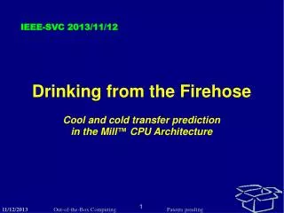
IEEE-SVC 2013/11/12 Drinking from the Firehose Cool and cold transfer prediction in the Mill™ CPU Architecture
The Mill Architecture Transfer prediction - without delay New with the Mill: Run-ahead prediction Prediction before code is loaded Explicit prefetch prediction No wasted instruction loads Automatic profiling Prediction in cold code addsx(b2, b5)
What is prediction? Prediction is a micro-architecture mechanism to smooth the flow of instructions in today’s slow-memory and long-pipeline CPUs. Like caches, the prediction mechanism and its success or failure is invisible to the program. Except in performance and power impact. Present prediction methods work quite well in small, regular benchmarks run on bare machines. They break down when code has irregular flow of control, and when processes are started or switched frequently.
The Mill CPU The Mill is a new general-purpose commercial CPU family. The Mill has a 10x single-thread power/performance gain over conventional out-of-order superscalar architectures, yet runs the same programs, without rewrite. • This talk will explain: • the problems that prediction is intended to alleviate • how conventional prediction works • the Mill CPU’s novel approach to prediction
Talks in this series Encoding The Belt Cache hierarchy Prediction Metadata and speculation Specification … You are here Slides and videos of other talks are at: ootbcomp.com/docs
Caution Gross over-simplification! This talk tries to convey an intuitive understanding to the non-specialist. The reality is more complicated.
Branches vs. pipelines if (I == 0) F(); else G(); load I eql 0 brfl lab call F … Do we call F() or G()? lab: call G … schedule decode cache execute 32 cycles (Intel Pentium 4 Prescott) 5 cycles (Mill)
Branches vs. pipelines if (I == 0) F(); else G(); load I eql 0 brfl lab call F … lab: call G … schedule decode cache execute call G stall stall stall eql 0 stall brfl stall load I stall More stall than work!
So we guess… if (I == 0) F(); else G(); Guess to call G (correct) load I eql 0 brfl lab call F … lab: call G … schedule decode cache execute inst inst inst inst inst load I inst brfl eql 0 call G inst Guess right? No stall!
So we guess… if (I == 0) F(); else G(); Guess to call F (wrong) load I eql 0 brfl lab call F … lab: call G … schedule decode cache execute eql 0 inst inst inst inst brfl inst load I call F inst inst Guess wrong? Mispredict stalls!
So we guess… if (I == 0) F(); else G(); Fix prediction: Call G load I eql 0 brfl lab call F … lab: call G … schedule decode cache execute call G inst inst inst inst inst inst inst stall stall stall stall stall stall stall Finally!
How the guess works if (I == 0) F(); else G(); load I eql 0 brfl lab call F … lab: call G … schedule decode cache execute
How the guess works if (I == 0) F(); else G(); load I eql 0 brfl lab call F … lab: call G … schedule decode cache execute call F load I eql 0 inst brfl
How the guess works if (I == 0) F(); else G(); load I eql 0 brfl lab call F … lab: call G … branch history table schedule decode cache execute inst call F brfl eql 0 load I
How the guess works if (I == 0) F(); else G(); load I eql 0 brfl lab call F … lab: call G … branch history table schedule decode cache execute inst inst inst stall stall brfl eql 0 load I call G Many fewer stalls!
So what’s it cost? • When (as is typical): • one instruction in eight is a branch • the predictor guesses right 95% of the time • the mispredict penalty is 15 cycles • predict failure wastes 8.5% of cycles Simplest fix is to lower the miss penalty. Shorten the pipeline! Mill pipeline is five cycles, not 15. Mill misprediction wastes only 3% of cycles
The catch - cold code The guess is based on prior history with the branch. What happens if there is no prior history? Cold code == random 50-50 guess • In cold code: • one instruction in eight is a branch • the predictor guesses right 50%of the time • the mispredict penalty is 15 cycles • predict failure wastes 48% of cycles • (23% on a Mill) Ouch!
But wait – it gets worse! Cold code means no relevant Branch History contents. It also means no relevant cache contents. DRAM branch history table 300+ cycles schedule decode cache execute inst brfl 15 cycles
Miss cost in cold code • In cold code, when: • one instruction in eight is a branch • the predictor guesses right 50% of the time • the mispredict penalty is 15 cycles • cache miss penalty is 300 cycles • cache line is 64 bytes, 16 instructions • cold misses waste 96% of cycles • (94% on a Mill) Ouch!
What to do? Use bigger cache lines Internal fragmentation means no gain Fetch more lines per miss Cache thrashing means no gain Nothing technical works very well.
What to do? Choose short benchmarks! No problem when benchmark is only a thousand instructions Blame the software! Code bloat is a software vendor problem, not a CPU problem Blame the memory vendor! Memory speed is a memory vendor problem, not a CPU problem This approach works. (for some value of “works”)
Fundamental problems Don’t know how much to load from DRAM. Mill knows how much will execute. Can’t spot branches until loaded and decoded. Mill knows where branches are, in unseen code Can’t predict spotted branches without history. Mill can predict in never-executed code. The rest of the talk shows how the Mill does this.
Extended Basic Blocks (EBBs) The Mill groups code into Extended Basic Blocks, single-entry multiple-exit sequences of instructions. Branches can only target EBB entry points; it is not possible to jump into the middle of an EBB. Execution flows through a chain of EBBs EBB branch EBB EBB Program counter EBB EBB chain
Predicting EBBs With an EBB organization, you don’t have to predict each branch. Only one of possibly many branches will pass control out of the EBB – so predict which one. EBB The Mill predicts exits, not branches. If control enters here - predict that control will exit here branch
Representing exits Code is sequential in memory and is held in cache lines which are also sequential inst inst inst inst inst inst inst inst
Representing exits There is one EBB entry point and one predicted exit point represented as the difference inst inst inst inst inst inst inst inst exit entry prediction
Representing exits There is one EBB entry point and one predicted exit point represented as the difference inst inst inst inst inst inst inst inst exit entry 3 2 line count inst count prediction Rather than a byte or instruction count, the Mill predicts: the number of cache lines the number of instructions in the last line
Representing exits Predictions also contain: • offset of the transfer target from the entry point • kind – jump, return, inner call, outer call jump 3 0xabcd 2 line count target offset inst count kind prediction “When we enter the EBB: fetch two lines, decode from the entry through the third instruction in the second line, and then jump to (entry+0xabcd)”
The Exit Table jump 3 0xabcd 2 line count target inst count kind
The Exit Table Predictions are stored in the hardware Exit Table exit table Capacity varies by Mill family member pred jump 3 0xabcd 2 line count target inst count kind • The Exit Table: • is direct-mapped, with victim buffers • is keyed by the EBB entry address and history info • has check bits to detect collisions • can use any history-based algorithm
Exit chains Starting with an entry point, the Mill can chain through successive predictions without actually looking at the code. entry address 123 123 returning the keyed prediction probe Exit Table using entry address as key 17 --- Exit Table
Exit chains Starting with an entry point, the Mill can chain through successive predictions without actually looking at the code. entry address 123 + add the offset to the EBB entry address to get the next EBB entry address ------------ 140 17 --- Exit Table
Exit chains Starting with an entry point, the Mill can chain through successive predictions without actually looking at the code. entry address • Repeat until: • no prediction in table • entry seen before (loop) • as far as you wanted to go 123 + rinse and repeat ------------ 140 140 + 17 -42 --- --- ------------ Exit Table 98
Prefetch Predictions chained from the Exit Table are prefetched from memory Prefetcher Exit Table pred Prefetches cannot fault or trap, instead stops chaining Prefetches are low priority, use idle cycles to memory line count entry addr Cache/DRAM
The Prediction Cache After prefetch, chain predictions are stored in the Prediction Cache Prediction cache Prefetcher pred The Prediction Cache is small, fast, and fully associative. Chaining from the Exit Table stops if a prediction is found to be already in the Cache, typically a loop. Chaining continues in the cache, possibly looping; a miss resumes from the Exit Table.
The Fetcher Predictions are chained from the Prediction Cache (following loops) to the Fetcher Prediction cache Prefetcher
The Fetcher Predictions are chained from the Prediction Cache (following loops) to the Fetcher Fetcher Prediction cache pred Lines are fetched from the regular cache hierarchy to a microcache attached to the decoder. entry addr line count Microcache Cache/DRAM
The Decoder Prediction chains end at the Decoder, which also receives a stream of the corresponding cache lines from the Microcache. Decoder Fetcher pred The result is that the Decoder has a queue of predictions, and another queue of the matching cache lines, that are kept continuously full and available. It can decode down the predicted path at the full 30+ instructions per cycle speed. Microcache
Timing Vertically aligned units work in parallel Prefetcher Fetcher Exit Table Decoder Prediction Cache Microcache 3 cycles 2 cycles 2 cycles 2 cycles mispredict penalty Once started, the predictor can sustain one prediction every three cycles from the Exit Table.
Fundamental problems redux Don’t know how much to load from DRAM. Mill knows how much will execute. Can’t spot branches until loaded and decoded. Mill knows where branches are, in unseen code Can’t predict spotted branches without history. Mill can predict in never-executed code.
Prediction feedback All predictors use feedback from execution experience to alter predictions to track changing program behavior. Exit Table Execute pred If a prediction was wrong, then it can be changed to predict what actually did happen. Exit Table contents reflects current history for all contained predictions.
“All contained predictions”? No! Not one prediction for each EBB in the program? • Tables are much to small to hold predictions for all EBBs. In a conventional branch predictor, each prediction is built up over time with increasing experience with the particular branch experience conventional branch table prediction Every process switch is followed by a period of poor predictions while experience is built up again. But if the CPU is switched to another process, the prediction is thrown away and overwritten.
A second source of predictions Like others, the Mill builds predictions from experience. However, it has a second source: the program load module. The load module is used when there is no experience. program load module code static data predictions exit table ? to decode key Missing predictions are read from the load module.
But there’s a catch… Loading a prediction from DRAM (or even L2 cache) takes much longer than a mispredict penalty! By the time it’s loaded we no longer need it! Solution: load bunches of likely-needed predictions program load module code static data predictions exit table key But – what predictions are likely-needed?
Likely-needed predictions No. Should we load on a misprediction? We have a prediction – it’s just wrong. No. Should we load on a missing prediction? It may only be a rarely-taken path that aged out of the table. We should bulk-load only when entering a whole new region of program activity that we haven’t been to before (recently), and may stay in for a while, or re-enter. Like a function.
Likely-needed predictions The Mill bulk-loads the predictions of a function when the call finds no prediction for the entry EBB. int main() { phase1(); phase2(); phase3(); return 0; } Each call triggers loading of the predictions for the code of that function. exit table
Program phase-change At phase change (or just code that was swapped out long enough): Recognize when a chain or misprediction leads to a call for which there is no Exit Table entry. Bulk load the predictions for the function. Start the prediction chain in the called function Chaining will prefetch the predicted code path Execute as fast as the code comes in. Overall delay: one load time for the first predictions one load time for the initial code prefetch two loads total - everything after that in parallel Vs. convential: one code load time perbranch
Where’s the load module get its predictions? The compiler can perfectly predict EBBs that contain no conditional branches. Calls, returns and jumps A profiler can measure conditional behavior. But instrumenting the load module changes the behavior. So the Mill does it for you. Exit table hardware logs experience with predictions. Post-processing of the log updates the load module. Log info is available for JITs and optimizers. Mill programs get faster every time they run.
The fine print Newly-compiled predictions assume every EBB will execute to the final transfer. This policy causes all cache lines of the EBB to be prefetched, improving performance at the expense of loading unused lines. Later experience corrects the line counts. When experience shows that an EBB in a function is almost never entered (often error code) then it is omitted from the bulk load list, saving Exit Table space and memory traffic.
Fundamental problem summary Don’t know how much to load from DRAM. Mill knows how much will execute. Can’t spot branches until loaded and decoded. Mill knows where the exits are. Can’t predict spotted branches without history. Mill can predict in never-executed code. Mill programs get faster every time they run.