Evaluation of Leading Parallel Architectures for Scientific Computing

1. Evaluation of Leading Parallel Architectures for Scientific Computing Leonid Oliker Future Technologies Group NERSC/LBNL www.nersc.gov/~oliker

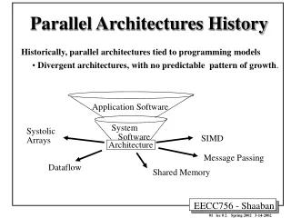
2. Overview • Success of parallel computing in solving large-scale practical applications relies on efficient mapping and execution on available architectures • Most real-life applications are complex, irregular, and dynamic • Generally believed that unstructured methods will constitute significant fraction of future high-end computing • Evaluate existing and emerging architectural platforms in the context of irregular and dynamic applications • Examine the complex interactions between high-level algorithms, programming paradigms, and architectural platforms.

3. Algorithms Architecturesand Programming Paradigms • Several parallel architectures with distinct programming methodologies and performance characteristics have emerged • Examined three irregular algorithms • N-Body Simulation, Dynamic Remeshing, Conjugate Gradient • Parallel Architectures • Cray T3E, SGI Origin2000, IBM SP, Cray (Tera) MTA • Programming Paradigms • Message-Passing, Shared Memory, Hybrid, Multithreading • Partitioning and/or ordering strategies to decompose domain • multilevel (MeTiS), linearization (RCM, SAW), combination (MeTiS+SAW)

4. Sparse Conjugate Gradient • CG oldest and best-known Krylov subspace method to solve sparse linear system (Ax = b) • starts from an initial guess of x • successively generates approximate solutions in the Krylov subspace & search directions to update the solution and residual • slow convergence for ill-conditioned matrices (use preconditioner) • Sparse matrix vector multiply (SPMV) usually accounts for most of the flops within a CG iteration, and is one of most heavily-used kernels in large-scale numerical simulations • if A is O(n) with nnz nonzeros, SPMV is O(nnz) but DOT is O(n) flops • To perform SPMV (yAx) • assume A stored in compressed row storage (CRS) format • dense vector x stored sequentially in memory with unit stride • Various numberings of mesh elements result in different nonzero patterns of A, causing different access patterns for x

5. Preconditioned Conjugate Gradient • PCG Algorithm Compute r0 = b - Ax0, p0 = z0 = M-1r0, for some initial guess x0 forj = 0, 1, …, until convergence j = (rj, zj) / (Apj, pj); xj+1 = xj + j pj; rj+1 = rj - aj Apj; zj+1 = M-1rj+1; bj = (rj+1, zj+1) / (rj, zj); pj+1 = zj+1 +bj pj; end for • Each PCG iteration involves • 1 SPMV iteration for Apj • 1 solve with preconditioner M (we consider ILU(0)) • 3 vector updates (AXPY) for xj+1, rj+1, pj+1 • 3 inner products (DOT) for update scalars j, bj • For symmetric positive definite linear systems, these conditions minimize distance between approximate and true solutions • For most practical matrices, SPMV and triangular solves dominate

6. Graph Partitioning Strategy: MeTiS • Most popular class of multilevel partitioners • Objectives • balance computational workload • minimize edge cut (interprocessor communication) • Algorithm • collapses vertices & edges using heavy-edge matching scheme • applies greedy partitioning algorithm to coarsest graph • uncoarsens it back using greedy graph growing + Kernighan-Lin Initial partitioning Refinementphase Coarseningphase

7. Linearization Strategy:Reverse Cuthill-McKee (RCM) • Matrix bandwidth (profile) has significant impact on efficiency of linear systems and eigensolvers • Geometry-based algorithm that generates a permutation so that non-zero entries are close to diagonal • Good preordering for LU or Cholesky factorization (reduces fill) • Improves cache performance (but does not explicitly reduce edge cut)

8. Linearization Strategy:Self-Avoiding Walks (SAW) • Mesh-based technique similar to space-filling curves • Two consecutive triangles in walk share edge or vertex (no jumps) • Visits each triangle exactly once, entering/exiting over edge/vertex • Improves parallel efficiency related to locality (cache reuse) and load balancing, but does not explicitly reduce edge cuts • Amenable to hierarchical coarsening & refinement Heber, Biswas, Gao: Concurrency: Practice & Experience, 12 (2000) 85-109

9. MPI Distributed-Memory Implementation • Each processor has local memory that only it can directly access; message passing required to access memory of another processor • User decides data distribution and organizes comm structure • Allows efficient code design at the cost of higher complexity • CG uses Aztec sparse linear library;PCG uses BlockSolve95 (Aztec does not have ILU(0) routine) • Matrix A partitioned into blocks of rows; each block to processor • Associated component vectors (x, b) distributed accordingly • Communication needed to transfer some components of x • AXPY (local computation); DOT (local sum, global reduction) • T3E (450 MHz Alpha processor, 900 Mflops peak, 245 MB main memory, 96 KB secondary cache, 3D torus interconnect)

10. SPMV Locality & Communication Statistics • Performance results using T3E hardware performance monitor • ORIG ordering has large edge cut (interprocessor communication) and poor data locality (high number of cache misses) • MeTiS minimizes edge cut; SAW minimizes cache misses

11. SPMV and CG Runtimes:Performance on T3E • Smart ordering / partitioning required to achieve good performance and high scalability • For this combination of apps & archs, improving cache reuse is more important than reducing interprocessor communication • Adaptivity will require repartitioning (reordering) and remapping

12. TriSolve and PCG Runtimes:Performance on T3E • Initial ordering / partitioning significant, even though matrix further reordered by BlockSolve95 • TriSolve dominates, and sensitive to ordering • SAW has slight advantage over RCM & MeTiS;an order faster than ORIG

13. (OpenMP) Shared-Memory Implementation • Origin2000 (SMP of nodes, each with dual 250 MHz R10000 processor & 512 MB local memory) • hardware makes all memory equally accessible from software perspective • non-uniform memory access time (depends on # hops) • each processor has 4 MB secondary data cache • when processor modifies word, all other copies of cache line invalidated • OpenMP-style directives (requires significantly less effort than MPI) • Two implementation approaches taken (identical kernels) • FLATMEM: assume Origin2000 has uniform shared-memory (arrays not explicitly distributed, non-local data handled by cache coherence) • CC-NUMA: consider underlying architecture by explicit data distribution • Each processor assigned equal # rows in matrix (block) • No explicit synchronization required since no concurrent writes • Global reduction for DOT operation

14. Origin2000 (Hardware Cache Coherency) Memory Directory Router Dir (>32P) Hub R12K R12K L2 Cache L2 Cache Node Architecture Communication Architecture

15. CG Runtimes:Performance on Origin2000 • CC-NUMA performs significantly better than FLATMEM • RCM & SAW reduce runtimes compared to ORIG • Little difference between RCM & SAW, probably due to large cache • CC-NUMA (with ordering) and MPI runtimes comparable, even though programming methodologies quite different • Adaptivity will require reordering and remapping

16. Hybrid (MPI+OpenMP) Implementation • Latest teraflop-scale systems designs contain large number of SMP nodes • Mixed programming paradigm combines two layers of parallelism • OpenMP within each SMP • MPI among SMP nodes • Allows codes to benefit from loop-level parallelism & shared-memory algorithms in addition to coarse-grained parallelism • Natural mapping to underlying architecture • Currently unclear if hybrid performance gains compensate for increased programming complexity and potential loss of portability • Incrementally add OpenMP directives to Aztec, and some code reorganization (including temp variables for correctness) • IBM SP (222 MHz Power3, 8-way SMP, current switch limits 4 MPI tasks per node)

17. CG Runtimes:Performance on SP • Intelligent orderings important for good hybrid performance • MeTiS+SAW best strategy, but not dramatically • For a given processor count, varying MPI tasks & OpenMP threads have little effect • Hybrid implementation does not offer noticeable advantage

18. Cray (Tera) MTA Multithreaded Architecture • 255 MHz MTA uses multithreading to hide latency (100-150 cycles per word) & keep processors saturated with work • no data cache • hashed memory mapping (data layout impossible) • near uniform data access from any processor to any memory location • Each processor has 128 hardware streams (32 registers & PC) • context switch on each cycle, choose next instruction from ready streams • a stream can execute an instruction only once every 21 cycles, even if no instructions reference memory • Synchronization between threads accomplished using full / empty bits in memory, allowing fine-grained threads • No explicit load balancing required since dynamic scheduling of work to threads can keep processor saturated • No difference between uni- and multiprocessor parallelism

19. MTA Multithreaded Implementation • Straightforward implementation (only requires compiler directives) • Special assertions used to indicate no loop-carried dependencies • Compiler then able to parallelize loop segments • Load balancing by OS (dynamically assigns matrix rows to threads) • Other than reduction for DOT, no special synchronization constructs required for CG • Synchronization required however for PCG • No special ordering required to achieve good parallel performance

20. SPMV and CG Runtimes:Performance on MTA • Both SPMV and CG show high scalability (over 90%) with 60 streams per processor • sufficient TLP to tolerate high overhead of memory access • 8-proc MTA faster than 32-proc Origin2000 & 16-proc T3E with no partitioning / ordering overhead; but will scaling continue beyond 8 procs? • Adaptivity does not require extra work to maintain performance

21. PCG Runtimes:Performance on MTA • Developed multithreaded version of TriSolve • matrix factorization times not included • use low-level locks to perform on-the-fly dependency analysis • TriSolve responsible for most of the computational overhead • Limited scalability due to insufficient TLP in our dynamic dependency scheme

22. CG Summary • Examined four different parallel implementations of CG and PCG using four leading programming paradigms and architectures • MPI most complicated • compared graph partitioning & linearization strategies • improving cache reuse more important than reducing communication • Smart ordering algorithms significantly improve overall performance • possible to achieve message passing performance using shared memory constructs through careful data ordering & distribution • Hybrid paradigm increases programming complexity with little performance gains • MTA easiest to program • no partitioning / ordering required to obtain high efficiency & scalability • no additional complexity for dynamic adaptation • limited scalability for PCG due to lack of thread level parallelism

23. 2D Unstructured Mesh Adaptation • Powerful tool for efficiently solving computational problems with evolving physical features (shocks, vortices, shear layers, crack propagation) • Complicated logic and data structures • Difficult to parallelize efficiently • Irregular data access patterns (pointer chasing) • Workload grows/shrinks at runtime (dynamic load balancing) • Three types of element subdivision

24. Parallel Code Development • Programming paradigms • Message passing (MPI) • Shared memory (OpenMP-style pragma compiler directives) • Multithreading (Tera compiler directives) • Architectures • Cray T3E  SGI Origin2000  Cray (Tera) MTA • Critical factors • Runtime • Scalability • Programmability • Portability • Memory overhead

25. Test Problem • Computational mesh to simulate flow over airfoil • Mesh geometrically refined 5 levels in specific regions to better capture fine-scale phenomena Serial Code 6.4 secs on 250 MHz R10K 14,605 vertices 28,404 triangles 488,574 vertices 1,291,834 triangles

26. Distributed-Memory Implementation • 512-node T3E (450 MHz DEC Alpha procs) • 32-node Origin2000 (250 MHz dual MIPS R10K procs) • Code implemented in MPI within PLUM framework • Initial dual graph used for load balancing adapted meshes • Parallel repartitioning of adapted meshes (ParMeTiS) • Remapping algorithm assigns new partitions to processors • Efficient data movement scheme (predictive & asynchronous) • Three major steps (refinement, repartitioning, remapping) • Overhead • Programming (to maintain consistent D/S for shared objects) • Memory (mostly for bulk communication buffers)

27. MESH ADAPTOR Edge Marking Coarsening Refinement Overview of PLUM INITIALIZATION LOAD BALANCER Initial Mesh Balanced? N Y Partitioning Repartitioning Mapping Reassignment Expensive? Y N FLOW SOLVER Remapping

28. Performance of MPI Code • More than 32 procs required to outperform serial case • Reasonable scalability for refinement & remapping • Scalable repartitioner would improve performance • Data volume different due to different word sizes

29. Shared-Memory Implementation • 32-node Origin2000 (250 MHz dual MIPS R10K procs) • Complexities of partitioning & remapping absent • Parallel dynamic loop scheduling for load balance • GRAPH_COLOR strategy (significant overhead) • Use SGI’s native pragma directives to create IRIX threads • Color triangles (new ones on the fly) to form independent sets • All threads process each set to completion, then synchronize • NO_COLOR strategy (too fine grained) • Use low-level locks instead of graph coloring • When thread processes triangle, lock its edges & vertices • Processors idle while waiting for blocked objects

30. Performance of Shared-Memory Code • Poor performance due to flat memory assumption • System overloaded by false sharing • Page migration unable to remedy problem • Need to consider data locality and cache effects to improve performance (require partitioning & reordering) • For GRAPH_COLOR • Cache misses15 M (serial) to85 M (P=1) • TLB misses7.3 M (serial) to53 M (P=1)

31. Multithreaded Implementation • 8-processor 250 MHz Tera MTA • 128 streams/proc, flat hashed memory, full-empty bit for sync • Executes pipelined instruction from different stream at each clock tick • Dynamically assigns triangles to threads • Implicit load balancing • Low-level synchronization variables ensure adjacent triangles do not update shared edges or vertices simultaneously • No partitioning, remapping, graph coloring required • Basically, the NO_COLOR strategy • Minimal programming to create multithreaded version

32. Performance of Multithreading Code • Sufficient instruction level parallelism exists to tolerate memory access overhead and lightweight synchronization • Number of streams changed via compiler directive

33. Schematic of Different Paradigms Distributed memory Shared memory Multithreading Before and after adaptation (P=2 for distributed memory)

34. Mesh Adaptation:Comparison and Conclusions • Different programming paradigms require varying numbers of operations and overheads • Multithreaded systems offer tremendous potential for solving some of the most challenging real-life problems on parallel computers

35. MPI SHMEM P0 P1 P0 P1 A A A A Put Send Receive Communication Library Communication Library Send-Receive pair Put or Get, not both Comparison of Programming Modelson Origin2000 CC-SAS P0 P1 A0 A1 A1 = A0 Load/Store We focus on adaptive applications (D-mesh, N-body)

36. Characteristics of the Model Transparency (for implementation) Increasing

37. INITIALIZATION Initial Mesh Partitioning FLOW SOLVER Matrix Transform Iterative Solver D-Mesh Algorithm MESH ADAPTOR LOAD BALANCER Edge Marking Balanced ? Y N Partitioning Refinement Re-mapping

38. P0 P0 P1 P1 P1 P1 MPI (physical partition): SAS (logical partition): Implementation of Flow Solver Matrix Transform: Easier in CC-SAS Iterative Solver: Conjugate Gradient, SPMV

39. Performance of Solver Most of the time is spent on iterative solver

40. P0 P0 P1 P1 P0 P0 P1 P1 Implementation of Load Balancer CC-SAS: MPI/SHMEM: Data Re-mapping in D-Mesh Logically partition Physically partition SAS provides substantial ease of programming in conceptual and orchestration level , far beyond implicit load/store vs. explicit messages

41. Performance of Adaptor CC-SAS suffers from the poor spatial locality of shared data

42. Performance of Load Balancer

43. Performance of D-Mesh CC-SAS suffers from poor spatial locality for smaller data sets CC-SAS benefits from the ease of programming for larger data sets

44. N-Body Simulation:Evolution of Two Plummer Bodies Barnes-Hut arises in many areas of science and engineering such as astrophysics, molecular dynamics, and graphics

45. N-Body Simulation (Barnes-Hut) Time Steps Build the Oct-tree Compute forces on all bodies Compute forces based on the tree Update body positions and velocities

46. MPI/SHMEM: “Locally Essential” Tree P0: Distribute/Collect Cells/Bodies N-Body:Tree Building Method CC-SAS: Shared Tree P0:

47. Performance of N-Body • For 16-processors, performance is similar • For 64-processors: • CC-SAS is better for smaller data sets • but worse for larger data sets

48. NBODY:Time Breakdown for (64P, 16K) Processor Identifier Less BUSY time for CC-SAS due to ease of programming

49. N-BODY:TIME BREAKDOWN (64P,1024K) Processor Identifier High MEM time for CC-SAS

50. N-Body :Improved Implementation SAS: Shared Tree Duplicate high-level cells MPI/SHMEM: Locally Essential Tree