Download
1 / 41
430 likes | 859 Views
Parallel Computing. George Mozdzynski April 2013. Outline. What is parallel computing? Why do we need it? Types of computer Parallel Computers today Challenges in parallel computing Parallel Programming Languages OpenMP and Message Passing Terminology.

E N D
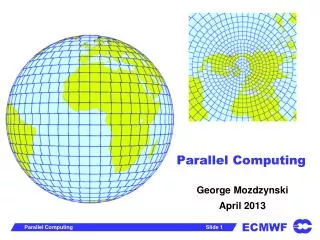
Parallel Computing George Mozdzynski April 2013 Parallel Computing
Outline • What is parallel computing? • Why do we need it? • Types of computer • Parallel Computers today • Challenges in parallel computing • Parallel Programming Languages • OpenMP and Message Passing • Terminology Parallel Computing
What is Parallel Computing? The simultaneous use of more than one processor or computer to solve a problem Parallel Computing
Why do we need Parallel Computing? • Serial computing is too slow • Need for large amounts of memory not accessible by a single processor Parallel Computing
An IFS T2047L149 forecast model takes about 5000 seconds wall time for a 10 day forecast using 128 nodes of an IBM Power6 cluster. How long would this model take using a fast PC with sufficient memory? (e.g. dual core Dell desktop) Parallel Computing
Ans. About 1 year This PC would also need ~2000 GBYTES of memory (8 GB is usual) 1 year is too long for a 10 day forecast! 5000 seconds is also too long … See www.spec.org for CPU performance data (e.g. Specfp2006) Parallel Computing
Some Terminology Hardware: CPU = Core = Processor = PE (Processing Element ) Socket = a chip with 1 or more cores (typically 2 or 4 today), more correctly the socket is what the chip fits into Software : Process (Unix/Linux) = Task (IBM) MPI = Message Passing Interface, standard for programming processes (tasks) on systems with distributed memory OpenMP = standard for shared memory programming (threads) Thread = some code / unit of work that can be scheduled (threads are cheap to start/stop compared with processes/tasks) User Threads = tasks * (threads per task) Parallel Computing
Measuring Performance • Wall Clock • Floating point operations per second (FLOPS or FLOP/S) • Peak (Hardware), Sustained (Application) • SI prefixes • Mega Mflops 10**6 • Giga Gflops 10**9 • Tera Tflops 10**12 ECMWF: 2 * 156 Tflops peak (P6) • Peta Pflops 10**15 2008-2010 (early systems) • Exa, Zetta, Yotta • Instructions per second, Mips, etc, • Transactions per second (Databases) Parallel Computing
S … … P P P P M M M Types of Parallel Computer P=Processor M=Memory S=Switch Shared Memory Distributed Memory Parallel Computing
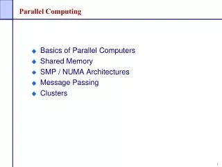
S … … P P P P … M M Node Node IBM Cluster (Distributed + Shared memory) P=Processor M=Memory S=Switch Parallel Computing
IBM Power7 Clusters at ECMWF This is just one of the TWO identical clusters Parallel Computing
…and one the world’s fastest (#3) and largest supercomputers – Fujitsu K computer 705,024 Sparc64 processor cores Parallel Computing
ORNL’s “Titan” System • #1 in Nov 2012 Top500 list • 18X peak perf. of ECMWF’s P7 clusters (C2A+C2B=1.5 Petaflops) • Upgrade of Jaguar from Cray XT5 to XK6 • Cray Linux Environment operating system • Gemini interconnect • 3-D Torus • Globally addressable memory • AMD Interlagos cores (16 cores per node) • New accelerated node design using NVIDIA K20 “Kepler” multi-core accelerators • 600 TB DDR3 mem. + 88 TB GDDR5 mem Source (edited): James J. Hack, Director, Oak Ridge National Laboratory
Types of Processor DO J=1,1000 A(J)=B(J) + C ENDDO LOAD B(J) FADD C STORE A(J) INCR J TEST Single instruction processes one element SCALAR PROCESSOR Single instruction processes many elements LOADV B->V1 FADDV V1,C->V2 STOREV V2->A VECTOR PROCESSOR Parallel Computing
Parallel Computers Today Higher #’s of cores => Less memory per core Less General Purpose CRAY XK6 Fujitsu K-Computer (Sparc) IBM BlueGeneQ More General Purpose Cray XE6 AMD Opteron Hitachi, Opteron HP 3000, Xeon IBM Power7 (e.g. ECMWF) Fujitsu, SPARC NEC SX8, SX9 SGI Xeon Sun, Opteron Bull, Xeon Performance Parallel Computing
The TOP500 project • started in 1993 • Top 500 sites reported • Report produced twice a year • EUROPE in JUNE (ISC13) • USA in NOV (SC13) • Performance based on LINPACK benchmark • dominated by matrix multiply (DGEMM) • HPC Challenge Benchmark • http://www.top500.org/ Parallel Computing
ECMWF in Top 500 TFlops KW Rmax – Tflop/sec achieved with LINPACK Benchmark Rpeak – Peak Hardware Tflop/sec (that will never be reached!) Parallel Computing
Why is Matrix Multiply (DGEMM) so efficient? VECTOR SCALAR / CACHE 1 n VL is vector register length VL FMA’s (VL + 1) LD’s (m * n) + (m + n) < # registers m * n FMA’s m + n LD’s VL m FMA’s ~= LD’s FMA’s >> LD’s Parallel Computing
NVIDIA Tesla C1060 GPU GPU programming • GPU – Graphics Processing Unit • Programmed using CUDA, OpenCL, OpenACC directives • High performance, low power, but ‘challenging’ to programme for large applications, separate memory, GPU/CPU interface (PCIX 8GB/sec) • Expect GPU technology to be more easily useable on future HPCs • http://gpgpu.org/developer • GPU hardware today supplied by • NVIDIA (Tesla) • INTEL (Xeon Phi) Parallel Computing
Key Architectural Features of a Supercomputer CPU Performance Parallel File-system Performance Interconnect Latency / Bandwidth MEMORY Latency / Bandwidth “a balancing act to achieve good sustained performance” Parallel Computing
What performance do Meteorological Applications achieve? • Vector computers • About 20 to 30 percent of peak performance (single node) • Relatively more expensive • Also have front-end scalar nodes (compiling, post-processing) • Scalar computers • About 5 to 10 percent of peak performance • Relatively less expensive • Both Vector and Scalar computers are being used in Met NWP Centres around the world • Is it harder to parallelize than vectorize? • Vectorization is mainly a compiler responsibility • Parallelization is mainly the user’s responsibility Parallel Computing
Challenges in parallel computing • Parallel Computers • Have ever increasing processors, memory, performance, but • Need more space (new computer halls = $) • Need more power (MWs = $) • Parallel computers require/produce a lot of data (I/O) • Require parallel file systems (GPFS, Lustre) + archive store • Applications need to scale to increasing numbers of processors, problems areas are • Load imbalance, Serial sections, Global Communications • Debugging parallel applications (totalview, ddt) • We are going to be using more processors in the future! • More cores per socket, little/no clock speed improvements Parallel Computing
Parallel Programming Languages? • OpenMP • directive based • support for Fortran 90/95/2003 and C/C++ • shared memory programming only • http://www.openmp.org • PGAS Languages (Partitioned Global Address Space) • UPC, Co-array Fortran (F2008) • One programming model for inter and intra node parallelism • MPI is not a programming language! Parallel Computing
Most Parallel Programmers use… • Fortran 90/95/2003, C/C++ with MPI for communicating between tasks (processes) • works for applications running on shared and distributed memory systems • Fortran 90/95/2003, C/C++ with OpenMP • For applications that need performance that is satisfied by a single node (shared memory) • Hybrid combination of MPI/OpenMP • ECMWF’s IFS uses this approach Parallel Computing
More Parallel Computing … Cache, Cache line Domain decomposition Halo, halo exchange Load imbalance Synchronization Barrier Parallel Computing
P P P C C2 C1 C1 M M Cache P=Processor C=Cache M=Memory Parallel Computing
P P P P P P P P C2 C2 C2 C2 C1 C1 C1 C1 C1 C1 C1 C1 IBM Power architecture (3 levels of $) C3 Memory Parallel Computing
Cache on scalar systems • Processors are 100’s of cycles away from Memory • Cache is a small (and fast) memory closer to processor • Cache line typically 128 bytes • Good for cache performance • Single stride access is always the best • Over inner loop leftmost index (fortran) BETTER DO J=1,N DO I=1,M A(I,J)= . . . ENDDO ENDDO WORSE DO J=1,N DO I=1,M A(J,I)= . . . ENDDO ENDDO Parallel Computing
IFS Grid-Point Calculations (an example of blocking for cache) NLON U(NGPTOT,NLEV) NGPTOT = NLAT * NLON NLEV = vertical levels Scalar NLAT Vector NLAT SUB GP_CALCS DO I=1,NPROMA ENDDO END DO J=1, NGPTOT, NPROMA CALL GP_CALCS ENDDO Lots of work Independent for each J Parallel Computing
Grid point space blocking for Cache Optimal use of cache / subroutine call overhead Parallel Computing
TL799 1024 tasks 2D partitioning 2D partitioning results in non-optimal Semi-Lagrangian comms requirement at poles and equator! Square shaped partitions are better than rectangular shaped partitions. arrival departure x x mid-point MPI task partition Parallel Computing
eq_regions algorithm Parallel Computing
2D partitioning T799 1024 tasks(NS=32 x EW=32) Parallel Computing
eq_regions partitioning T799 1024 tasks N_REGIONS( 1)= 1 N_REGIONS( 2)= 7 N_REGIONS( 3)= 13 N_REGIONS( 4)= 19 N_REGIONS( 5)= 25 N_REGIONS( 6)= 31 N_REGIONS( 7)= 35 N_REGIONS( 8)= 41 N_REGIONS( 9)= 45 N_REGIONS(10)= 48 N_REGIONS(11)= 52 N_REGIONS(12)= 54 N_REGIONS(13)= 56 N_REGIONS(14)= 56 N_REGIONS(15)= 58 N_REGIONS(16)= 56 N_REGIONS(17)= 56 N_REGIONS(18)= 54 N_REGIONS(19)= 52 N_REGIONS(20)= 48 N_REGIONS(21)= 45 N_REGIONS(22)= 41 N_REGIONS(23)= 35 N_REGIONS(24)= 31 N_REGIONS(25)= 25 N_REGIONS(26)= 19 N_REGIONS(27)= 13 N_REGIONS(28)= 7 N_REGIONS(29)= 1 Parallel Computing