Download
1 / 57
570 likes | 642 Views
Role of Bidomain Model of Cardiac Tissue in the Dynamics of Phase Singularities. Jianfeng Lv Advisor: Sima Setayeshgar May 15, 200 9. Outline. Motivation Numerical Implementation Numerical Results Conclusions and Future Work. Motivation:. Patch size: 5 cm x 5 cm Time spacing: 5 msec.

E N D
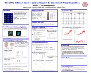
Role of Bidomain Model of Cardiac Tissue in the Dynamics of Phase Singularities Jianfeng Lv Advisor: Sima Setayeshgar May 15, 2009
Outline • Motivation • Numerical Implementation • Numerical Results • Conclusions and Future Work
Motivation: Patch size: 5 cm x 5 cm Time spacing: 5 msec • Ventricular fibrillation (VF) is the main cause of sudden cardiac death in industrialized nations, accounting for 1 out of 10 deaths. • Strong experimental evidence suggests that self-sustained waves of electrical wave activity in cardiac tissue are related to fatal arrhythmias. • And … the heart is an interesting arena for applying the ideas of pattern formation. [1] W.F. Witkowski, et al., Nature 392, 78 (1998)
Spiral Waves and Cardiac Arrhythmias • Transition from ventricular tachycardia to fibrillation is conjectured to occur as a result of breakdown of a single spiral (scroll) into a spatiotemporally disordered state, resulting from various mechanisms of spiral (scroll) wave instability. [1] Tachychardia Fibrillation Courtesy of Sasha Panfilov, University of Utrecht Goal is to use analytical and numerical tools to study the dynamics of reentrant waves in the heart on physiologically realistic domains. [1] A. V. Panfilov, Chaos 8, 57-64 (1998)
Cardiac Tissue Structure Cells are typically 30 – 100 µm long 8 – 20 µm wide Propagation Speeds = 0.5 m / s = 0.17 m / s Guyton and Hall, “Textbook of Medical Physiology” Nigel F. Hooke, “Efficient simulation of action potential propagation in a bidomain”, 1992
Cable Equation and Monodomain Model • Early studies used the 1-D cable equation to describe the electrical behavior of a cylindrical fiber. transmembrane potential: • intra- (extra-) cellular potential: • transmembrane current (per unit length): axial currents: ionic current: • conductivity tensor: capacitance per unit area of membrane: resistances (per unit length): Adapted from J. P. Keener and J. Sneyd, Mathematical Physiology
Bidomain Model of Cardiac Tissue The bidomain model treats the complex microstructure of cardiac tissue as a two-phase conducting medium, where every point in space is composed of both intra- and extracellular spaces and both conductivity tensors are specified at each point.[1-3] From Laboratory of Living State Physics, Vanderbilt University [1] J. P. Keener and J. Sneyd, Mathematical Physiology [2] C. S. Henriquez, Critical Reviews in Biomedical Engineering21, 1-77 (1993) [3] J. C. Neu and W. Krassowska, Critical Reviews in Biomedical Engineering21, 137-1999 (1993)
Bidomain Model Transmembrane current: Transmembrane current: Ohmic axial currents: Conservation of total currents:
Conductivity Tensors • The ratio of the intracellular and extracellular conductivity tensors; Bidomain: Monodomain: Cardiac tissue is more accurately described as a three-dimensional anisotropic bidomain, especially under conditions of applied external current such as in defibrillation studies.[1-2] [1] B. J. Roth and J. P. Wikswo, IEEE Transactions on Biomedical Engineering41, 232-240 (1994) [2] J. P. Wikswo, et al., Biophysical Journal 69, 2195-2210 (1995)
Monodomain Reduction By setting the intra- and extra-cellular conductivity matrices proportional to each other, the bidomain model can be reduced to monodomain model. (1) Substitute (1) into If , then we obtain the monodomain model.
Rotating Anisotropy Local Coordinate Lab Coordinate From Streeter, et al., Circ. Res. 24, p.339 (1969)
Scroll Twist Solutions Scroll Twist, Fz Twist Twist Rotating anisotropy generated scroll twist, either at the boundaries or in the bulk.
Significance? In isotropic excitable media (a = 1), for twist > twistcritical, straight filament undergoes buckling (“sproing”) instability [1] What happens in the presence of rotating anisotropy (a > 1)?? Henzi, Lugosi and Winfree, Can. J. Phys. (1990).
Filament Tension Destabilizing or restabilizing role of rotating anisotropy!!
Phase Singularity • Tips and filaments are phase singularities that act as organizing centers for spiral (2D) and scroll (3D) dynamics, respectively.
Focus of this work • Analytical and numerical works[1-5] have been done on studying the dynamic of scroll waves in monodomain in the presence of rotating anisotropy . • Rotating anisotropy can induce the breakdown of scroll wave; • Rotating anisotropy leads to “twistons”, eventually destabilizing scroll filament; • The focus of this work is computational study of the role of rotating anisotropy on the dynamics of phase singularities in bidomain model of cardiac tissue as a conducting medium. [1] Biktashev, V. N. and Holden, A. V. Physica D 347, 611(1994) [2] Keener, J. P. Physica D 31, 269 (1988) [3] S. Setayeshgar and A. J. Bernoff, PRL 88, 028101 (2002) [4] A. V. Panfilov and J. P. Keener, Physica D 84, 545 (1995) [5] Fenton, F. and Karma, A. Chaos 8, 20 (1998):
Numerical Implementation of the Bidomain Equations with Rotating Anisotropy
Governing Equations Governing equations describing the intra- and extracellular potentials: • Transmembrane potential propagation • Conservation of total current • : transmembrane potential • : intra- (extra-) cellular potential • :ionic current • : conductivity tensor in intra- (extra-) cellular space
Ionic current models • Ionic current, , described by a FitzHugh-Nagumo-like kinetics [1] These parameters specify the fast processes such as initiation of the action potential. The refractoriness of the model is determined by the function . [1] A. V. Panfilov and J. P. Keener, Physica D 84, 545-552 (1995)
Boundary conditions • No-flux boundary conditions: Let For a rectangular, Normal vector to the domain boundary: Conductivity tensors in natural frame:
Numerical Implementation • Numerical solution of parabolic PDE (for Vm ) Forward Euler scheme: Crank-Nicolson scheme: The spacial operator is approximated by the finite difference matrix operator
Numerical Implementationcont’d • Numerical solution of elliptic PDE (for Ve ) Direct solution of the resulting systems of linear algebraic equations by LU decomposition. ai , bi , ci , mi are coefficients of terms after discretization of LHS. denotes the extracellular potential Ve on node (x=i, y=j, z=k). denotes the corresponding RHS after discretization.
Numerical Implementationcont’d • Index re-ordering to reduce size of band-diagonal system Elements ai, bi, ci … are constants obtained in finite difference approximation to the elliptic equation.
Numerical Convergence A time sequence of a typical action potential with various time-steps. The figures show that time step δt = 0.01 is suitable taking both efficiency and accuracy of computation into account.
Filament-finding algorithm “Distance” between two tips: If two tips are not on a same fiber surface or on adjacent surfaces, the distance is defined to be infinity. Otherwise, the distance is the distance along the fiber surface Search for the closest tip
Filament-finding algorithm “Distance” between two tips: If two tips are not on a same fiber surface or on adjacent surfaces, the distance is defined to be infinity. Otherwise, the distance is the distance along the fiber surface Make connection
Filament-finding algorithm “Distance” between two tips: If two tips are not on a same fiber surface or on adjacent surfaces, the distance is defined to be infinity. Otherwise, the distance is the distance along the fiber surface Continue doing search
Filament-finding algorithm “Distance” between two tips: If two tips are not on a same fiber surface or on adjacent surfaces, the distance is defined to be infinity. Otherwise, the distance is the distance along the fiber surface Continue
Filament-finding algorithm “Distance” between two tips: If two tips are not on a same fiber surface or on adjacent surfaces, the distance is defined to be infinity. Otherwise, the distance is the distance along the fiber surface Continue
Filament-finding algorithm “Distance” between two tips: If two tips are not on a same fiber surface or on adjacent surfaces, the distance is defined to be infinity. Otherwise, the distance is the distance along the fiber surface Continue
Filament-finding algorithm “Distance” between two tips: If two tips are not on a same fiber surface or on adjacent surfaces, the distance is defined to be infinity. Otherwise, the distance is the distance along the fiber surface The closest tip is too far
Filament-finding algorithm “Distance” between two tips: If two tips are not on a same fiber surface or on adjacent surfaces, the distance is defined to be infinity. Otherwise, the distance is the distance along the fiber surface Reverse the search direction
Filament-finding algorithm “Distance” between two tips: If two tips are not on a same fiber surface or on adjacent surfaces, the distance is defined to be infinity. Otherwise, the distance is the distance along the fiber surface Continue
Filament-finding algorithm “Distance” between two tips: If two tips are not on a same fiber surface or on adjacent surfaces, the distance is defined to be infinity. Otherwise, the distance is the distance along the fiber surface Complete the filament
Filament-finding algorithm “Distance” between two tips: If two tips are not on a same fiber surface or on adjacent surfaces, the distance is defined to be infinity. Otherwise, the distance is the distance along the fiber surface Start a new filament
Filament-finding algorithm “Distance” between two tips: If two tips are not on a same fiber surface or on adjacent surfaces, the distance is defined to be infinity. Otherwise, the distance is the distance along the fiber surface Repeat until all tips are consumed
Numerical ResultsFilament dynamics of Bidomain • Examples of filament-finding results used to characterize breakup. Total filament length(grid points) Filament number Time (s) Time (s) Total filament length(grid points) Filament number Time (s) Time (s)
Numerical Resultsof previous work in Monodomain • Previous study has shown rotating anisotropy can induce the breakdown of scroll wave.[1] Model size : 60x60x9 for 10mm thickness No break-up while the fiber rotation is less then 60o or total thickness is less than 3.3mm. Iso surfaces of 3D view of scroll wave in the medium with = 0.1111 [1] A. V. Panfilov and J. P. Keener, Physica D 84, 545-552 (1995)
Results of computational experiments with different parameters of cardiac tissue. Numerical Results Bidomain/Monodomain Comparison For ∆x=0.5, the size of rectangular grid is 60x60x9 points For ∆x=0.2, the size of rectangular grid is 150x150x23 points [1] A. V. Panfilov and J. P. Keener Physica D 1995
Numerical Results:Larger Domain Size Result Contour plots of transmembrane potential selected tissue layers at t = 750 time units. Scroll wave breakup is evident in the middle layers. Filament number Time (s) Total filament length(grid points) Model size: 140x294x48; ∆x = ∆y = ∆z = 0.25 (space units) Time step: ∆t = 0.01 (time units) ; Time (s)
Conclusions so far … • We have numerically implemented electrical wave propagation in the bidomain model of cardiac tissue in the presence of rotating anisotropy using FHN-like reaction kinetics. • In the finer monodomain model and bidomain model, the boundaries of irregular behavior shift; • Numerical Limitation: • Large space step in previous study causes mesh effect; • Model size is too small. Increasing model size in bidomain model is limited by the physical memory;
Multigrid Techniques:Multigrid Hierarchy Relax Interpolate Restrict Relax Relax Relax Relax Dragica Vasileska, “Multi-Grid Method”
Multigrid Techniques: Multigrid method Structure of multigrid cycles • Coarse-grid correction • Compute the defect on the fine grid; • Restrict the defect; • Solve exactly on the coarse grid for the correction; • Interpolate the correction to the fine grid; • Compute the next approximation • Relaxation “Numerical Recipes in C”, 2nd Editoin S denotes smoothing; E denotes exact solution on the finest grid. Descending line \ denotes restriction, each ascending line / denotes prolongation. William L. Briggs, “A Multigrid Tutorial”
Multigrid Techniques: Full Multigrid Algorithm • Multigrid method starts with some initial guess on the finest grid and carries out enough cycles to achieve convergence. Efficiency can be improved by using the Full Multigrid Algorithm (FMG) FMG with the exact solution at the coarsest level. It uses V-cycles (W-cycles) as the solver on each grid level. “Numerical Recipes in C”, 2nd Editoin