Download
1 / 55
570 likes | 738 Views
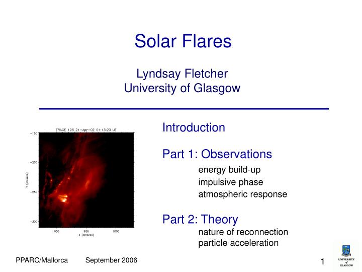
Solar Flares. Lyndsay Fletcher University of Glasgow. Introduction Part 1: Observations energy build-up impulsive phase atmospheric response Part 2: Theory nature of reconnection particle acceleration. RHESSI and TRACE flare observations. Bremsstrahlung emission: 12-25keV – Red

E N D
Solar Flares Lyndsay Fletcher University of Glasgow Introduction Part 1: Observations energy build-up impulsive phase atmospheric response Part 2: Theory nature of reconnection particle acceleration 1
RHESSI and TRACE flare observations Bremsstrahlung emission: 12-25keV – Red 25-50keV – Blue Thermal emission at ~ 1.5MK and ~25MK, green 2
Flare Questions • What is the source of the flare energy? • How is energy stored and how/why is it released? • How is energy converted into heat, particles, radiation, bulk kinetic energy? • How does the solar atmosphere respond? 3
Introduction Part 1: Observations energy build-up impulsive phase atmospheric response Part 2: Theory nature of reconnection particle acceleration 4
Source of Flare Energy Energy is imparted to the coronal magnetic field at or below photosphere - photosphere is a high beta plasma so gas pressure forces dominate. magnetic field evolution from SOHO/MDI 5
Energy storage in the corona MHD version of Ampère’s Law j = B/m Twisting the field produces ‘free energy’ in the form of current. MHD Force balance equation Assume ~ steady state, with negligible gravitational forces and pressure gradients (low beta corona). Then Force-free condition, i. e. field and current are aligned So , meaning a constant along field lines 6
When does energy build-up occur? Does the magnetic field emerge already bearing free energy? From vector magnetic field measurements, Leka et al. (1996) determined the curl of the magnetic field in an emerging active region They also measured the photospheric flows during and after emergence. Result: AR twists are too large to be generated by the photospheric flows. So the field emerges from the convection zone already carrying current. 7
Location of free energy - observations Shear is concentrated close to magnetic neutral line 8
Can flares be predicted? Folk Knowledge: A complex, rapidly-evolving, large active region has highest probability of producing a flare, within a few days of its emergence. More accurate predictions? Prediction based on past X-ray activity (Bayesian statistics) Moderately successful (Wheatland 2004) Statistics of magnetic field parameters and their variations Rather unsuccessful (Leka and Barnes 2006) Neural Net ‘learning’ of appearance of ARs about to flare Underway 9
Preflare Activity What are the signs that a flare is going to happen? Most Reliable - The rise/darkening/expansion of an AR Ha filament minutes to hours before flare (Svestka 1976, Martin 1980) 10
Filaments are dense, cool gas suspended in the corona. The slow filament rise probably indicates the onset of an MHD instability. polar crown filament active region filament movie movie 11
Preflare Activity Are there any other signs that a flare is going to happen? Other pre-flare phenomena include: • Small UV/EUV ‘twinkles’ (Moore & Sterling, Warren & Warshall) • Small GOES events and preheating • “Sigmoid” magnetic configuration (Hudson & Sterling) • Early hard X-ray coronal sources (Lin et al.) • Moving blueshifted Ha events (Des Jardins & Canfield 2003) But none of these is unique to flares 12
Energy storage and flare trigger - overview • Magnetic energy for the flare is stored as field-aligned currents. • Most of the energy is concentrated close to a neutral line, probably low in the atmosphere (~10,000km). • The flare is related to the onset of an MHD instability, probably followed by fast magnetic reconnection. • The conditions leading to a flare cannot easily be identified – flare prediction is still not possible. 13
Introduction Part 1: Observations energy build-up impulsive phase atmospheric response Part 2: Theory nature of reconnection particle acceleration 14
GOES flare classification scheme Flux in the 1-8 Å band C: more than 10-6 W m-2 at Earth (e.g. C4.2 flare => 4.2x10⁻⁶ Wm-2) M: more than 10-5 W m-2 at Earth X: more than 10-4 W m-2 at Earth Flare X-ray Time Profiles • Impulsive phase - energy release • Hard X-rays (10s of keV) • Duration ~ 5 minutes to 1 hour • Bursty time profile (tacc ~ seconds) • Gradual phase - response • thermal emission (~0.1-1 keV) • rise time ~ minutes 15
hot thermal emission Non-thermal electron bremsstrahlung: I(e) ~ e-g Impulsive Phase X-ray Spectrum Gamma-ray lines 16
X-Rays X-rays observed by e.g. RHESSI are electron-proton bremsstrahlung from energetic electrons (> 15keV) • Thermal bremsstrahlung: Eelectron ~ E target and spectrum F(e)~ e-e/kt • - Primarily coronal. • Non-thermal bremsstrahlung: Eelectron >> E target and spectrum F(e)~e-g • - Primarily chromospheric ‘thick target’ (electron slows as it radiates) • - Very inefficient: ~ 10-5 of the electron energy radiated as X-rays. 17
RHESSI X-ray imaging • 2” imaging at ~ 20-50 keV, ~ 4s resolution (if sufficient counts) • Spectroscopy with 1 keV energy resolution Orange = 25-50keV Blue = TRACE white light 20” =15,000km RHESSI imaging 18
10 100 E (keV) X-Ray spectrum • In impulsive phase, HXR spectrum can be fitted by a hot (20MK) or superhot (~60MK) thermal component plus a power-law F(E)=FoE-g. • Parameters of fit are correlated and vary during flare. • Microflares also show thermal + power-law spectrum. electron spectral index Typical spectral fit, Holman et al (2003) Variation of fit parameters during a flare, Grigis & Benz (2005) 19
No photospheric albedo correction With albedo correction HXR spectral inversion Photon spectrum I() is related to source-averaged electron spectrum If Q is known, the integral can be inverted (i.e. differentiated) to recover source-averaged spectrum (Kontar et al. ’03, ’06) Collisional thick target interpretation Beam number ~ 1036-37 e- s-1 above 20keV Combining with observed HXR footpoint areas < 10” x 10” Beam flux > 1018-19e- cm-2 s-1 above 20keV 20
Other Impulsive Phase Emission During the impulsive phase bursts of g-rays hard X-rays, UV/EUV, Ha and (sometimes) optical emission show where fast particles hit the low atmosphere 1600 A broadband emission HXR contours on 195A emission Optical/UV/EUV emission from heat deposition /ionisation / collisional / radiative excitation White light luminosity increase confirmstotal energy input deduced from HXRs White light footpoints 21
Separatrix intersections What is significant about footpoint locations? Radiation from non-thermal particles appears at the photospheric intersection of separatrix surfaces (eg Demoulin, Aulanier). Motion of footpoints across magnetic field can be used to deduce a coronal magnetic reconnection rate. Time evolution of HXR footpoint positions Metcalf et al. (2003) 22
Separatrices (2-D and 3-D) Separatrices are (curves)/surfaces separating domains of different magnetic connectivity in (2D)/3D Radiation produced at predicted separatrix locations shows the importance of reconnection processes happening at domain boundaries (Priest and Schrijver 1999) (Priest and Schrijver 1999) 23
hot thermal emission Non-thermal electron bremsstrahlung: I(e) ~ e-g Flare Impulsive Phase Energy Spectrum Gamma-ray lines 24
Production of nuclear de-excitation lines Gamma-rays • Continuumg-rays by bremsstrahlung (~ 10MeV) • Nuclear de-excitation lines caused by • proton bombardment; • - ‘prompt’ radiation provides a diagnostic • of protons above 30MeV • The positron annihilation line at 511keV • The neutron capture line at 2.23 MeV - n(p,g)D • - this is a delayed line, as neutrons must slow down before reacting. • formed low in the atmosphere, and after other emissions. 25
Location of g-ray sources Similar time profiles for HXRs and de-excitation lines imply related acceleration. However, radiation produced by ions is in a different location from electron bremsstrahlung Neutrons produced by energetic ions (10s of MeV/nucleon). The capture line is predicted to form within 500km of neutron production site. But observed to be systematically offset from HXRs (electrons) by ~ 10,000km (15”). Hurford et al. 2006 26
above 20 -40keV Flare Energy Budget Estimates made by Emslie et al. (2004, 2005) confirm that a significant fraction of total flare energy appears in fast particles 27
Coronal radio emission Metric and decimetric Type III bursts are plasma radiation produced by electron beams (mode-conversion of Langmuir waves). Upward and downward-going beams observed Occur at peak time of HXR emission. Detailed radio/HXR burst-to-burst time-correlations improve at higher starting frequency (Benz et al ‘05) Non-linear coherent emission electron number estimates difficult. Microwave gyro-synchrotron emission from fast electrons in coronal loops is also significant. Electron numbers can be made to agree with numbers from HXR. Also info on angular distribution 28
50-100 keV 20-30 keV 30-50 keV Coronal Hard X-ray Sources • First observed by SMM/HXIS, then at better resolution by Yohkoh/HXT. Now in many RHESSI flares (inc. occulted) • Flares seen without HXR footpoints – only coronal HXR loops. Emission up to 50keV implies ne ~ 1011cm-3(Veronig & Brown 2004) Occulted sources present up to at least 50 keV (Bone et al. 2006) Coronal energy deposition between 1030 and 1031 erg 29
14-April-2002, 22:25 UT 10 d WIND/3DP, =2.6 d <F(E)>, RHESSI, =2.5 1 d F (E), RHESSI, =4.5 0 0.1 0.01 Electron Flux 1E-3 1E-4 1E-5 10 100 Energy, keV In situ electron measurements Some hard X-ray events are also observed by particle detectors in space (e.g. 14 Apr 2002, Krucker et al, 2003) In situ electron fluxes do not agree with thick-target fluxes deduced from RHESSI
Impulsive phase – main points • During the impulsive phase, most of the flare energy is released. • Energetic particles receive up to 50% of the total energy (rest goes to CME and heating). • Most of the impulsive phase energy is focused into a few small sources. • These sources are closely related to magnetic separatrices. • Up to 1037 electrons accelerated per second (i.e. all the electrons in (10,000km)3 at 1010 cm-3. • Similar number of ions accelerated, but in a different place or following a different path. 31
Introduction Part 1: Observations energy build-up impulsive phase atmospheric response Part 2: Theory nature of reconnection particle acceleration 32
loops then cool through EUV temperatures Atmospheric response – soft X-ray and EUV Flare leads to brightening coronal loops, producing high fluxes of soft X-ray emission (0.1-1 keV). 33
Atmospheric response - chromospheric upflows Energy input in the form of a beam heats the chromosphere rapidly and – if heating is strong enough - it expands upwards. Chromospheric ‘evaporation’ has been observed spectroscopically in Ha(e.g. Antonucci et al 1984) Also in UV/EUV using SoHO/CDS post-flare observations (e.g. Czaykowska et al 1999) Blueshifts on outer part of arcade are evaporation Redshifts on inner part of arcade are material cooling and draining. 34
Latest numerical simulations disagree with evaporation scenario Coronal density increases, but temperature does not: increasing ionisation, radiative losses and gas expansion absorb the energy T ne Allred et al 2006. 35
Introduction Part 1: Observations energy build-up impulsive phase atmospheric response Part 2: Theory nature of reconnection particle acceleration 36
Liberation of stored energy Magnetic reconnection allows the coronal field to reconfigure, liberating magnetic energy Reconnection is the process whereby two field lines, being frozen in and carried along by the fluid, break and rejoin in a different way. A B So a particle that was on fieldline A can end up on fieldline B Reconnection results from the local breakdown of flux conservation. 37
Breakdown of Flux Conservation The induction equation – describes advection and dissipation of field Define associated timescales : ta = L/v andtd = L2/h where L is the typical length scale for variation in the magnetic field. The ratio oftd to tais called the Magnetic Reynolds number, RM Normally in the corona, dissipation is much slower than advection (low collisional resistivityh, large v and L); so the field is frozen. 38
Magnetic Field Dissipation td in the corona is about 106 years. How do we speed up dissipation? td = L2/h so must decrease the length scale L, or increase resistivity. As field is advected by flow, it generates steep gradients - current sheets V Field lines are advected in to the current sheet, reconnect, and plasma is advected out at the upstream Alfvén speed - Sweet-Parker reconnection. Sweet-Parker reconnection is rather inefficient: the rate scales as Rm-1/2 It is too slow (by ~ 5 orders of mag) to explain flare energy release. 39
Petschek Reconnection The Petschek model reduces the size of the diffusion region. Reconnection rate increases as plasma is ‘slingshotted’ out Outflow at ~ Alfvèn speed • The reconnection rate is determined by the external conditions • At slow shocks, energy conversion can occur • May be fast enough to explain flare release if a high ‘anomalous resistivity’ is invoked. 40
Non-MHD regimes of reconnection Most solar reconnection theory is done in the MHD framework. MHD Ohm’s law This only includes a resistivity term due to classical (Ohmic) dissipation. Generalised Ohm’s law • e.g. the Hall term arises since protons and electrons follow different orbits in a magnetic field • Decoupling of e, p leads to whistler wave generation • Dissipation occurs by wave-particle interaction 41
2-D versus 3-D reconnection Simple models are 2D. The corona is certainly 3D (Priest and Schrijver 1999) (Priest and Schrijver 1999) 42
Introduction Part 1: Observations energy build-up impulsive phase atmospheric response Part 2: Theory nature of reconnection particle acceleration 43
Mechanisms of Particle Acceleration • Accelerating coronal charged particles requires electric fields. • There are three mechanisms most often discussed in the context of • acceleration of solar flare particles • DC field acceleration - E large-scale and organised • Stochastic resonant acceleration – E small-scale and random • Diffusive Shock Acceleration – Both large and small-scale fields • The last of these three is generally thought of as a ‘secondary’ accelerator • of particles, in the presence of a shock associated with a coronal mass • ejection. We shall concentrate on the DC and stochastic models. 44
electron beam FE FDRAG Field-aligned DC electric fields • For example, a local increase in resistivity in a current loop leads to • large potential drop (since huge inductance of circuit prevents rapid • change in current) • Electrons accelerated if this DC field is greater than the Dreicer field,Ed • The Dreicer field is the value of the DC field such that the force exerted • on the electrons exceeds drag force from e-e Coulomb collisions • Ed typically 10-4 V/cm • Electrons with speeds greater than a critical speed =vTe (Ed/E)1/2 are • freely accelerated ‘runaway’ electrons B 45
E L~109cm total potential drop = 1010 V! DC electric fields in a current sheet • Observations suggest that super-Dreicer fields occur in reconnection regions. • Inferred values of reconnection electric field are ~ 1 V/cm • In a model with symmetry in the plane perpendicular to the loop, this field is • parallel to solar surface and • normal to loops in post-flare arcade Problem: E B almost everywhere, so mostly particles EB drift. However, near X-line, there may be an unmagnetised region (B(x,y) 0) - or a component of B parallel to E So some efficient particle acceleration can occur – how much? 46
Stochastic Resonant Acceleration Particles gyrating in a magnetic field pick up energy from plasma waves if their gyration frequency is resonant with (multiples of) the wave frequency Frequency matching condition: w-k|| v|| - lW/g = 0 However, as soon as a particle picks up some energy from a monochromatic wave, its gyration frequency changes and resonance is lost. But particles resonating with a wave spectrum can ‘hop’ stochastically from one resonance to another as their energy increases or decreases (e.g. Miller & Vinas 1993, Miller 1998) , = wave and cyclotron frequencies k|| = parallel wave number v|| = parallel particle speed l = integer 47
Energy vs. time for a single proton in isotropic, high frequency turbulence Energy lost or gained in each interaction, but overall, the energy of the particle increases Protons and ions (mostly) resonate with high-frequency Alfvenic waves Electrons resonate with electron cyclotron waves Miller & Viñas (1993) 48
Closing Thoughts • Observations of solar flares in the X-ray and EUV, from the last 15 years • or so, have demonstrated a great variety and complexity • To a great extent, they still support the overall picture of reconnection in the • corona resulting in the acceleration of a vast number of particles, which lead • to heating and mass-motion in the lower atmosphere. • However, the study of solar flares involves some formidable theoretical • problems, such as: • What is the microphysics of coronal reconnection? • How do we extend our understanding of 2-D reconnection to 3-D? • How do we tie together the MHD, plasma and kinetic aspects of theory? • We must also not ignore the physics which has been painfully learned in other • fields, such as lab devices and magnetospheric reconnection 49
11:04 11:06 11:08 11:10 11:12 11:14 RHESSI preflare sources RHESSI often observes X-rays at ~ 10-20 keV, several minutes before the impulsive phase. 50