Download
1 / 49
1k likes | 1.92k Views
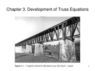
Chapter 4. Development of Beam Equations. Recall: Truss (or bar) elements are subjected to axial tensile or compressive forces only (no bending) and deform by change in length Beam elements (Chapter 4) - deform by bending

E N D
Chapter 4. Development of Beam Equations • Recall: • Truss (or bar) elements are subjected to axial tensile or compressive forces only (no bending) and deform by change in length • Beam elements (Chapter 4) - deform by bending • Frame elements (Chapter 5) – combined axial, bending, and torsional deformation
Review – Beam Theory M – moment distribution E – Young’s modulus I – Moment of Inertia of cross-section v – transverse displacement V – shear load w – distributed load
Beam Theory (cont.) If EI = constant and only concentrated loads and moments are applied, i.e. w(x)=0 Solution (exact)
Steps in the Finite Element Method • Discretize the region and select element type • Select a displacement function • Define the strain/displacement and stress/strain relations • Derive the element equations • Direct Stiffness Method • Energy Methods • Method of Weighted Residuals (Galerkin’s method) • Assemble global equations and impose boundary conditions • Solve for unknown nodal displacements • Solve for element strains and stresses • Interpret results
Step 1 – Select Element Type Beam Element
Step 2 – Select Displacement Function Note: Which satisfies the governing differential equation exactly if EI = constant and only concentrated loads and moments are applied. Otherwise, the finite element solution is an approximation.
Step 2 – Select Displacement Function (cont.) • Displacement parameters a1, a2, a3 and a4 have no physical meaning • Rewrite displacement function in terms of nodal displacements and rotations
Step 2 – Select Displacement Function (cont.) Solve for ai, i = 1,4 Substitute into:
Step 2 – Select Displacement Function (cont.) Matrix form:
Beam Element Interpolation Functions % % Matlab code to plot beam interpolation functions % D. G. Taggart - Spring 2009 close all; clear all; clc; % L=1; x=linspace(0,L,25); N1=(2*x.^3-3*x.^2*L+L^3)/L^3; N2=(x.^3*L-2*x.^2*L^2+x*L^3)/L^3; N3=(-2*x.^3+3*x.^2*L)/L^3; N4=(x.^3-x.^2*L)/L^3; % subplot(2,2,1) plot(x,N1) title('N_1(x)') % subplot(2,2,2) plot(x,N2) title('N_2(x)') % subplot(2,2,3) plot(x,N3) title('N_3(x)') % subplot(2,2,4) plot(x,N4) title('N_4(x)')
Step 3 – Strain-displacement & stress-strain relations Kinematic assumption from beam theory – “plane sections remain planar and normal to the midplane” Strain – displacement relation Moment – displacement relation Shear force – displacement relation (neglecting shear deformation)
Step 3 – Derive element equations (direct approach) Recall Consider f1yand m1
Step 3 – Derive element equations (cont.) Similarly for f2y and m2 Matrix form
P A Simple Example – Cantilever Beam Beam theory: FEA (single element): => =>
Timoshenko Beam Theory (includes transverse shear deformation) See text for derivation where (ksA) is the shear area and G is the shear modulus
Steps 5-8 – Examples (several in text)Problem 4-2, p. 166 Note: Could use symmetry, consider full model first
Example 4-2 - Global Equations BC’s: d1y = 1 = d3y = d5y = 5 = 0 Loads:F2y = F4y = -10,000 lb, M2 = M3 = M4 = 0 Need to solve system of 5 equations
Example 4-2 (cont.) • Matlab Command Window output: • d = • -0.0480 • -0.0000 • 0.0000 • -0.0480 • -0.0000 • Matlab: • E=30e6; • I=500; • L=10*12; • K=(E*I/L^3)*[24 0 6*L 0 0 ; • 0 8*L^3 2*L^2 0 0 ; • 6*L 2*L^2 8*L^2 -6*L 2*L^2 ; • 0 0 -6*L^2 24 0 ; • 0 0 2*L^2 0 8*L^2 ]; • F=[-10000; 0 ; 0 ; -10000; 0]; • d=K\F Note: 2 = 3 = 4 = 0
Example 4-2 (cont.) Or, using symmetry: 2 = 3 = 4 = 0 which yields Solving d2y=d4y=-.048 in
5,000 lb 10 ft Example 4-2 (cont.) Third approach
25,000 lb-ft 25,000 lb-ft 5000 lb 5000 lb Example 4-2 (cont.) Element loads and moments (element 1) Note: equilibrium is satisfied
Beam Elements – Distributed Loading Consider a beam with fixed supports subjected to a uniform distributed load
Beam with fixed supports & uniform distributed load For this statically indeterminate beam, it can be shown that the reaction forces and moments are: Hence, we can replace the distributed loading by an equivalent set of concentrated forces and moments:
Work equivalent forces & moments Work done by distributed loads:
Recall For uniform loading: Work done: Equivalent concentrated forces and moments Work done by distributed loads
Work equivalent concentrated forces and moments(Appendix D – cont.)
Example 4.6, p. 179 Single element solution with d1y = 1 = 0
Example 4.6 (cont.) Solving Reaction forces: Concentrated forces and moments due to distributed loads Text calls this term F(e) (effective global nodal forces)
E = 30 x 106 psi I = 100 in4 Comparison to Exact Solution Beam theory solution:
Comparison of beam theory to one element FEA:Displacement distribution
Comparison of beam theory to one element FEA:Moment distribution
Comparison of beam theory to one element FEA:Shear force distribution
Potential energy • Strain energy • Potential energy of external forces Beam element equations derived using potential energy approach Recall:
Strain Energy – including only bending stresses (neglects shear deformation) where
Strain Energy – (cont.) and Strain energy:
Element Stiffness Matrix Hence (same result as from Direct Stiffness Method)
Potential energy of external forces (cont.) Work equivalent concentrated forces and moments
Potential Energy – Beam Element Minimization of p gives (see Appendix A, pp. 714 - 715) where
Galerkin’s Method – Beam Element Recall the governing differential equation of a beam Approximate solutions Galerkin’s method Where Ni’s are the beam element interpolation functions “Residual”
Galerkin’s Method (cont.) Substituting and integrating by parts twice yields see text for details