Download
1 / 28
280 likes | 403 Views
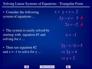
Chapter 4 Systems of Linear Equations; Matrices. Section 1 Review: Systems of Linear Equations in Two Variables. Opening Example.

E N D
Chapter 4Systems of Linear Equations; Matrices Section 1 Review: Systems of Linear Equations in Two Variables
Opening Example A restaurant serves two types of fish dinners- small for $5.99 and large for $8.99. One day, there were 134 total orders of fish, and the total receipts for these 134 orders was $1,024.66. How many small fish dinners and how many large fish dinners were ordered?
Systems of Two Equations in Two Variables • We are given the linear system ax + by = h cx + dy = k A solution is an ordered pair (x0, y0) that will satisfy each equation (make a true equation when substituted into that equation). The solution set is the set of all ordered pairs that satisfy both equations. In this section, we wish to find the solution set of a system of linear equations. To solve a system is to find its solution set.
Solve by Graphing • One method to find the solution of a system of linear equations is to graph each equation on a coordinate plane and to determine the point of intersection (if it exists). The drawback of this method is that it is not very accurate in most cases, but does give a general location of the point of intersection. Lets take a look at an example: • Solve the following system by graphing: 3x + 5y = –9 x+ 4y = –10
Solve by GraphingSolution 3x + 5y = –9 x+ 4y = –10 First line (intercept method) If x = 0, y= –9/5 If y = 0 , x = –3 Plot points and draw line (2, –3) Second line: Intercepts are (0, –5/2) , ( –10,0) From the graph we estimate that the point of intersection is (2,–3). Check: 3(2) + 5(–3)= –9 and 2 + 4(–3)= –10. Both check.
Another Example • Now, you try one: • Solve the system by graphing: 2x + 3 = y x + 2y = –4
Another ExampleSolution • Now, you try one: • Solve the system by graphing: 2x + 3 = y x + 2y = –4 We can do this on a graphing calculator by first solving the second equation for y to get y = –0.5x – 2 If we enter both of these equations into the calculator and find the intersection point we get the screen shown. The solution is (–2,–1).
Method of Substitution • Although the method of graphing is intuitive, it is not very accurate in most cases, unless done by calculator. There is another method that is 100% accurate. It is called the method of substitution. This method is an algebraic one. It works well when the coefficients of x or y are either 1 or –1. For example, let’s solve the previous system 2x + 3 = y x + 2y = -4 using the method of substitution.
Method of Substitution(continued) The steps for this method are as follows: • Solve one of the equations for either x or y. • Substitute that result into the other equation to obtain an equation in a single variable (either x or y). • Solve the equation for that variable. • Substitute this value into any convenient equation to obtain the value of the remaining variable.
2x + 3 = y x + 2y = –4 x + 2(2x + 3) = –4 x + 4x + 6 = –4 5x + 6 = –4 5x = –10 x = –2 Substitute y from first equation into second equation Solve the resulting equation After we find x = –2, then from the first equation, we have 2(–2) + 3 = y or y = –1. Our solution is (–2, –1) Example(continued)
Solve the system using substitution: 3x – 2y = 7 y = 2x – 3 Another Example
Solve the system using substitution: 3x – 2y = 7 y = 2x – 3 Solution: Another Example Solution
Basic Terms • A consistent linear system is one that has one or more solutions. • If a consistent system has exactly one solution (unique solution), it is said to be independent. An independent system will occur when the two lines have different slopes. • If a consistent system has more than one solution, it is said to be dependent. A dependent system will occur when the two lines have the same slope and the same y intercept. In other words, the graphs of the lines will coincide. There will be an infinite number of points of intersection. Two systems of equations are equivalent if they have the same solution set.
Basic Terms • An inconsistent linear system is one that has no solutions. This will occur when two lines have the same slope but different y intercepts. In this case, the lines will be parallel and will never intersect. • Example: Determine if the system is consistent, independent, dependent or inconsistent: 2x – 5y = 6 –4x + 10y = –1
Solution of Example • Solve each equation for y to obtain the slope intercept form of the equation: • Since each equation has the same slope but different y intercepts, they will not intersect. This is an inconsistent system.
Elimination by Addition • The method of substitution is not preferable if none of the coefficients of x and y are 1 or –1. For example, substitution is not the preferred method for the system below: 2x – 7y = 3 –5x + 3y = 7 • A better method is elimination by addition. The following operations can be used to produce equivalent systems: • Two equations can be interchanged. • An equation can be multiplied by a non-zero constant. • A constant multiple of one equation and is added to another equation.
Elimination by AdditionExample • For our system, we will seek to eliminate the x variable. The coefficients are 2 and –5. Our goal is to obtain coefficients of x that are additive inverses of each other. • We can accomplish this by multiplying the first equation by 5, and the second equation by 2. • Next, we can add the two equations to eliminate the x-variable. • Solve for y • Substitute y value into original equation and solve for x • Write solution as an ordered pair
Solve 2x – 5y = 6 –4x + 10y = –1 Elimination by AdditionAnother Example
Solve 2x – 5y = 6 –4x + 10y = –1 Solution: 1. Eliminate x by multiplying equation 1 by 2 . 2. Add two equations 3. Upon adding the equations, both variables are eliminated producing the false equation 0 = 11 Elimination by AdditionAnother Example 4. Conclusion: If a false equation arises, the system is inconsistent and there is no solution.
Application • A man walks at a rate of 3 miles per hour and jogs at a rate of 5 miles per hour. He walks and jogs a total distance of 3.5 miles in 0.9 hours. How long does the man jog?
Application • A man walks at a rate of 3 miles per hour and jogs at a rate of 5 miles per hour. He walks and jogs a total distance of 3.5 miles in 0.9 hours. How long does the man jog? • Solution: Let x represent the amount of time spent walking and y represent the amount of time spent jogging. Since the total time spent walking and jogging is 0.9 hours, we have the equation x + y = 0.9. We are given the total distance traveled as 3.5 miles. Since Distance = Rate x Time, distance walking = 3x and distance jogging = 5y. Then total distance is 3x + 5y= 3.5.
We can solve the system using substitution. 1. Solve the first equation for y 2. Substitute this expression into the second equation. 3. Solve second equation for x 4. Find the y value by substituting this x value back into the first equation. 5. Answer the question: Time spent jogging is 0.4 hours. Solution: Application(continued)
Supply and Demand The quantity of a product that people are willing to buy during some period of time depends on its price. Generally, the higher the price, the less the demand; the lower the price, the greater the demand. Similarly, the quantity of a product that a supplier is willing to sell during some period of time also depends on the price. Generally, a supplier will be willing to supply more of a product at higher prices and less of a product at lower prices. The simplest supply and demand model is a linear model where the graphs of a demand equation and a supply equation are straight lines.
Supply and Demand(continued) In supply and demand problems we are usually interested in finding the price at which supply will equal demand. This is called the equilibriumprice, and the quantity sold at that price is called the equilibrium quantity. If we graph the the supply equation and the demand equation on the same axis, the point where the two lines intersect is called the equilibrium point. Its horizontal coordinate is the value of the equilibrium quantity, and its vertical coordinate is the value of the equilibrium price.
Supply and DemandExample Example: Suppose that the supply equation for long-life light bulbs is given by p = 1.04 q – 7.03, and that the demand equation for the bulbs is p = –0.81q + 7.5 where q is in thousands of cases. Find the equilibrium price and quantity, and graph the two equations in the same coordinate system.
Supply and Demand(Example continued) If we graph the two equations on a graphing calculator and find the intersection point, we see the graph below. Demand Curve Supply Curve Thus the equilibrium point is (7.854, 1.14), the equilibrium price is $1.14 per bulb, and the equilibrium quantity is 7,854 cases.
Now, Solve the Opening Example • A restaurant serves two types of fish dinners- small for $5.99 each and large for $8.99. One day, there were 134 total orders of fish, and the total receipts for these 134 orders was $1024.66. How many small dinners and how many large dinners were ordered?
Solution • A restaurant serves two types of fish dinners- small for $5.99 each and large for $8.99. One day, there were 134 total orders of fish, and the total receipts for these 134 orders was $1024.66. How many small dinners and how many large dinners were ordered? • Answer: 60 small orders and 74 large orders