Download

1 / 37
410 likes | 653 Views
FIT ANALYSIS IN RASCH MODEL. University of Ostrava Czech republic 26-31, March, 2012. Two questions relating fit analysis :. How to assess fit the real data to the chosen model of measurement? What should we do if the data don’t fit the model?. Two approaches to assessing fit.

E N D
FIT ANALYSIS IN RASCH MODEL University of Ostrava Czech republic 26-31, March, 2012
Two questions relating fit analysis: • How to assess fit the real data to the chosen model of measurement? • What should we do if the data don’t fit the model?
Two approaches to assessing fit • Fit statistics, based on standardized residuals • Chi – square criteria, assesssing the closeness of model and empirical characteristic curves
Letani be a scored response for the interaction of the person n, n=1,…,N,and the item i, i=1,…,I(the 1’s and 0’s in dichotomous case); xni– standardized residual; Pni– the probability of a correct response for person n on item i.
Properties of standardized residuals xni M(xni)=0, D(xni)=1; In theory values vary in range (-∞,+∞); in practice values usually range from -10 to +10. If Pni=0,99 andani=0 thanxni≈-9,94 ; similarily if Pni=0,01 and ani=1, than xni≈ 9,94 ; Positive values represent correct responses: xni>0ifani=1; Negative values represent incorrect responses: xni<0 ifani=0; The values are assumed to have normal distributionN (0,1).
Dependence of the standardized residual on the difference θn - δi
Statistics xnican have positive and negative values, so summing residuals across items and persons is informative. The solution of this problem is squaring standadized residuals:
Properties of yni Statistics ynihas only non negative values; In theory values yni vary in range (0,+∞); in practice values usually range from0 to 100, at that most of values are in range (0,2); The expected value and variance of yniare: M(yni)=1, D(yni)=2. Statistics yni=xni2can be evaluated as having χ2distribution with one degree of freedom.
Distribution features of statistics yni These squared standardized residuals are only approximate chi-squares Statistics yniwould have exact χ2distribution, if the following conditions were completed: 1)aniwas continuous variable (rather than discrete); 2) exact values of the possibity Pniwere known (indeed only estimates of this possibility are known that are based on parameter estimates); 3) The data fit the measurement model.
Person fit statistics for an examinee n: This statistics is a sum of all values ynifor the examinee across all items. It has approximately χ2distribution with df=I. A problem: for each degree of freedom there is a different crirical value, so no single critical value can be used
Item fit statistics for an item i: This statistics is a sum of all values ynifor the item across all examinees. It has approximately χ2distribution with df=N. The same problem: for each degree of freedom there is a different crirical value, so no single critical value can be used.
A possible solution of the critical value problem Transformating the chi-squre statistics into a mean –square by dividing the chi-square by its degrees of freedom (Outfit MNSQ in Winsteps): Person-fit statistics for an examinee n: Item-fit statistics for an item i :
Properties of mean square statistics Un(1)andUi(1) Statistics Un(1)и Ui(1)vary in range from [0,+∞); Expected value is 1: M(Un(1))=M(Ui(1))=1. Statistics Un(1)и Ui(1)are very sensitive to outliers (unexpected correct or incorrect responses).
To counteract this sentivity to outliers the weighted versions of person-fit and item-fit statistics were developed:
Properties of weighted fit statistics Each squared standardized residual yniis weighted by the dispersion D(ani)=Pni·qnibefore it is summed. The value D(ani) is the least for the items difficulty of which don’t correspond to ability level of the examinee. Thus, contribution of these items to statistics Un(2)andUi(2)will be reduced. Statistics Un(2)andUi(2)vary in range [0,+∞) and have expected value of 1.
Total fit statistics The MNSQ statistics Un(1), Un(2), Ui(1) иUi(2)are called total fit statistics. Observed values of MNSQ statisticsUn(1), Un(2), Ui(1)andUi(2)are the more closed to expected value 1, the more the real data fir the Rasch model. If the real data don’t fit the model, observed values of MNSQ statisticswill differ from 1.
The problem with critical values of total fit statistics Critical values of mnsq statistics are different for different samples and different tests The distributions of mnsq statistics are approximate and, as a rule, empirical distributions differ from the theoretical ones So we can not use the same critical values for mnsq statistics defined from their theoretical distribution.
Interpretation of total fit statistics values The value of item-fit ststistics of 1.3 can be interpreted as indicating noise in the data in the item response pattern: there is 30% more variation in the data than it was predicted by the modal (underfit) The value of item-fit ststistics of 0.8can be interpreted as indicating Guttman pattern: there is 20% less variation in the data than it was predicted by the modal (overrfit)
Transformating the mnsq statistics to standardized form (zstd in Winsteps) There are two kinds of transformation that converts the mean-square to an approximate t-statistics: Logarithm transformation Cube-root transformation
Properties of standardized fit statistics Standardized fit statistics thave approximately normal distribution N(0,1), So with this statistics common critical values can be developed: for significance level 0,05 the acceptable values are in the range of (-2,+2) Simulation studies have shown that the standardized fit statistics have more consistent distributional properties in the face of varying sample size than do the mnsq ststistics
Statistics for Item Fit Analysis Total item-fit statistics Ui(1) (Mnsq Outfit) Standardized item-fit statistics ti(1) (Zstd Outfit) Weighted total item-fit statistics Ui(2)(Mnsq Infit) Standardized weighted item-fit statistics ti(2) (Zstd Infit) A combination of item-fit statistics provides the best opportunity to detect poor fit items
Recommended ranges for the total item-fit statistics for different test types
Some reasons for poor item-fit (underfit - mnsq fit-statistics values are more than 1.2; zstd fit-statistics values are more than +2) Test is not unidimensional Bed items (mistakes with keys, bed distractors in MC items, item mistakes, etc.) Particular features of examinee behavior (guessing, carelessness, etc.)
About items that are overfit (mnsq fit-statistics values are less than 0.8; zstd fit-statistics values are less than -2) Patterns of these items are too perfect (Guttman). It is not in agreement with a probabilistic nature of the model Too perfect patterns of these items can be consequence of more high discrimination of these items. A possible reason for it is violation of local independence: examinee’s response to one item affects his response to another one. Such items don’t contribute into measurement of ability.
The second approach to item fit: chi-square statistics df=s - 1
Problems with chi-square approach use How many points for sample dividing should we take? 3 or 5 or 10 or more? In many test situations this statistics has low efficiency In Rasch measurement the preference gives to item-fit statistics described above. In addition software Winsteps produces confidence intervals for ICC based on chi-square approach
Example of fit analysis: test description Test contains 50 items which are divided into three parts: part 1 has 32 MC items with 4 options (А1 – А32); part 2 has 12 opened items with a short answer (В1 – В12);part 3 has 6 items with free-constructed response (С1 – С6)/ Most of items were scored dichotomously, and a few items were scored polytomously. The total sample size is 655.
ICC of a poor fit item Dicriminating power of this item is lower than other items have
ICC of an item with two fit statistics with values below the left critical value Discriminating power of the item is higher than other items have
Statistics for Person Fit Analysis Total person-fit statistics Un(1) (Mnsq Outfit) Standardized person-fit statistics tn(1) (Zstd Outfit) Weighted total person-fit statistics Un(2)(Mnsq Infit) Standardized weighted person-fit statistics tn(2) (Zstd Infit) A combination of person-fit statistics provides the best opportunity to detect poor fit items
Some reasons of poor person fit: Bed items Personal features of the examinee Gap in the examinee knowledge Violation of test conditions