Download
1 / 63
630 likes | 820 Views
Multiple testing in large-scale gene expression experiments. Lecture 22, Statistics 246, April 13, 2004. Outline. Motivation & examples Univariate hypothesis testing Multiple hypothesis testing Results for the two examples Discussion. Motivation.

E N D
Multiple testing in large-scale gene expression experiments Lecture 22, Statistics 246, April 13, 2004
Outline • Motivation & examples • Univariate hypothesis testing • Multiple hypothesis testing • Results for the two examples • Discussion
Motivation SCIENTIFIC: To determine which genes are differentially expressed between two sources of mRNA (trt, ctl). STATISTICAL: To assign appropriately adjusted p-values to thousands of genes, and/or make statements about false discovery rates. I will discuss the issues in the context of two experiments, one which fits the aims above, and one which doesn’t, but helps make a number of points.
Apo AI experiment (Matt Callow, LBNL) Goal. To identify genes with altered expression in the livers of Apo AI knock-out mice (T) compared to inbred C57Bl/6 control mice (C). • 8 treatment mice and 8 control mice • 16 hybridizations: liver mRNA from each of the 16 mice (Ti , Ci ) is labelled with Cy5, while pooled liver mRNA from the control mice (C*) is labelled with Cy3. • Probes: ~ 6,000 cDNAs (genes), including 200 related to lipid metabolism.
Golub et al (1999) experiments Goal. To identify genes which are differentially expressed in acute lymphoblastic leukemia (ALL) tumours in comparison with acute myeloid leukemia (AML) tumours. • 38 tumour samples: 27 ALL, 11 AML. • Data from Affymetrix chips, some pre-processing. • Originally 6,817 genes; 3,051 after reduction. Data therefore a 3,051 38 array of expression values. Comment: this wasn’t really the goal of Golub et al.
Data The gene expression data can be summarized as follows treatment control X = Here xi,j is the (relative) expression value of gene i in sample j. The first n1 columns are from the treatment (T); the remaining n2 = n - n1 columns are from the control (C).
Steps to find diff. expressed genes • Formulate a single hypothesis testing strategy • Construct a statistic for each gene • Compute the raw p-values for each gene by permutation procedures or from distribution models • Consider the multiple testing problem a. Find the maximum # of genes of interest b. Assign a significance level for each gene
Univariate hypothesis testing Initially, focus on one gene only. We wish to test the null hypothesis H that the gene is not differentially expressed. In order to do so, we use a two sample t-statistic:
p-values The p-value or observed significance levelp is the chance of getting a test statistic as or more extreme than the observed one, under the null hypothesis H of no differential expression. Although the previous test statistic is denoted by t, it would be unwise to assume that its null distribution is that of Student’s t. We have another way to assign p-values which is more or less valid: using permutations.
Computing p-values by permutations We focus on one gene only. For the bth iteration, b = 1, , B; Permute the n data points for the gene (x). The first n1 are referred to as “treatments”, the second n2 as “controls”. For each gene, calculate the corresponding two sample t-statistic, tb. After all the B permutations are done; Put p = #{b: |tb| ≥ |t|}/B (plower if we use >). With all permutations in the Apo AI data, B = n!/n1!n2! = 12,870; for the leukemia data, B = 1.2109 .
Many tests: a simulation study Simulation of this process for 6,000 genes with 8 treatments and 8 controls. All the gene expression values were simulated i.i.d from a N (0,1) distribution, i.e. NOTHING is differentially expressed in our simulation. We now present the 10 smallest raw (unadjusted) permutation p-values.
Discussion At this point in the lecture we discussed the following question: what assumptions on the null distributions of the gene expression values xi = (xi,1 , xi,2 , …xi,n) are necessary or sufficient for the permutation-based p-values just described to be valid? And, are they applicable in our examples? First, we figured out that p-values are valid if their distribution is uniform(0,1) under the null hypothesis. Secondly, we concluded that if the null distribution of xi is exchangeable, i.e. invariant under permutations of 1,…,n, then, we could reasonably hope (and actually prove) that the distribution of the permutation-based p-values is indeed uniform on 1,…,n. We also noted that having the joint distribution i.i.d. would be sufficient, as this implied exchangeability. Next, we considered the ApoAI experiment. Because the 16 log-ratios for each gene involved a term from the pooled control mRNA, called C* above, it seems clear that an i.i.d. assumption is unreasonable. Had the experiment been carried out by using pooled control mRNA from mice other than the controls in the experiment, an exchangeability assumption under the null hypothesis would have been quite reasonable. Unfortunately, C* did come from the same mice as the Ci, so exchangeability is violated, and the assumption is at best an approximation.
Unadjusted p-values Clearly we can’t just use standard p-value thresholds of 05 or .01.
Multiple testing: Counting errors Assume we are testing H1, H2, , Hm . m0 = # of true hypotheses R = # of rejected hypotheses V = # Type I errors [false positives] T= # Type II errors [false negatives]
Type I error rates • Per comparison error rate (PCER): the expected value of the number of Type I errors over the number of hypotheses, • PCER = E(V)/m. • Per-family error rate (PFER): the expected number of Type I errors, • PFER = E(V). • Family-wise error rate: the probability of at least one type I error • FEWR = pr(V ≥ 1) • False discovery rate (FDR) is the expected proportion of Type I errors among the rejected hypotheses • FDR = E(V/R; R>0) = E(V/R | R>0)pr(R>0). • Positive false discovery rate (pFDR): the rate that discoveries are false • pFDR = E(V/R | R>0).
Multiple testingFamily-wise error rates • FWER = Pr(# of false discoveries >0) • = Pr(V>0) Bonferroni (1936) Tukey (1949) Westfall and Young (1993) discussed resampling ……
FWER and microarrays Two approaches for computing FWER maxT step-down procedure Dudoit et al (2002) Westfall et al (2001) minP step-down procedure Ge et al (2003), a novel fast algorithm
Multiple testingFalse discovery rates Q is set to be 0 when R=0 FDR = expectation of Q = E(V/R; R>0) Seeger (1968) Benjamini and Hochberg (1995)
Caution with FDR • Cheating: Adding known diff. expressed genes reduces FDR • Interpreting: FDR applies to a set of genes in a global sense, not to individual genes
Some previous work on FDR Benjamini and Hochberg (1995) Benjamini and Yekutieli (2001) Storey (2002) Storey and Tibshirani (2001) ……
Types of control of Type I error • strong control:control of the Type I error whatever the true and false null hypotheses. For FWER, strong control means controlling • max pr(V≥ 1 | M0) • M0H0C • where M0 = the set of true hypotheses (note |M0| = m0); • exact control: under M0 , even though this is usually unknown. • weak control: control of the Type I error only under the complete null hypothesisH0C = iHi . For FWER, this is control of pr( V ≥ 1 | H0C ).
Adjustments to p-values For strong control of the FWER at some level , there are procedures which will take m unadjusted p-values and modify them separately, so-called single step procedures, the Bonferroni adjustment or correction being the simplest and most well known. Another is due to Sidák. Other, more powerful procedures, adjust sequentially, from the smallest to the largest, or vice versa. These are the step-up and step-down methods, and we’ll meet a number of these, usually variations on single-step procedures. In all cases, we’ll denote adjusted p-values by , usually with subscripts, and let the context define what type of adjustment has been made. Unadjusted p-values are denoted by p.
What should one look for in a multiple testing procedure? As we will see, there is a bewildering variety of multiple testing procedures. How can we choose which to use? There is no simple answer here, but each can be judged according to a number of criteria: Interpretation: does the procedure answer a relevant question for you? Type of control: strong, exact or weak? Validity: are the assumptions under which the procedure applies clear and definitely or plausibly true, or are they unclear and most probably not true? Computability: are the procedure’s calculations straightforward to calculate accurately, or is there possibly numerical or simulation uncertainty, or discreteness?
p-value adjustments: single-step • Define adjusted p-values π such that the FWER is controlled at level where Hiis rejected when πi≤ . • Bonferroni: πi = min (mpi, 1) • Sidák: πi = 1 - (1 - pi)m • Bonferroni always gives strong control, proof next page. • Sidák is less conservative than Bonferroni. When the genes are independent, it gives strong control exactly (FWER= ), proof later. It controls FWER in many other cases, but is still conservative.
Proof for Bonferroni(single-step adjustment) pr (reject at least one Hiat level | H0C) = pr (at least one i≤ | H0C) ≤ 1m pr (i≤ | H0C) , by Boole’s inequality = 1m pr (Pi≤ /m | H0C), by definiton of i = m /m , assuming Pi ~ U[0,1]) =. Notes: 1. We are testing m genes, H0C is the complete null hypothesis, Piis the unadjusted p-value for gene i , while ihere is the Bonferroni adjusted p-value. 2. We use lower case letters for observed p-values, and upper case for the corresponding random variables.
Proof for Sidák’s method(single-step adjustment) pr(reject at least one Hi | H0C) = pr(at least onei≤ | H0C) = 1 - pr(alli> | H0C) = 1-∏i=1m pr(i > | H0C) assuming independence Here iis the Sidák adjusted p-value, and so i > if and only if Pi > 1-(1- )1/m (check), giving 1-∏i=1m pr(i > | H0C) = 1-∏i=1m pr(Pi > 1-(1- )1/m | H0C) = 1- { (1- )1/m }m since all Pi ~ U[0,1], =
Single-step adjustments (ctd) The minP method of Westfall and Young: i= pr( min Pl≤ pi | H) 1≤l≤m Based on the joint distribution of the p-values {Pl }. This is the most powerful of the three single-step adjustments. If Pi U [0,1], it gives a FWER exactly = (see next page). It always confers weak control, and gives strong control under subset pivotality (definition next but one slide).
Proof for (single-step) minP adjustment Given level a, let ca be such that pr(min1 ≤i ≤m Pi≤ ca| H0C) =a . Note that {i≤ } {Pi ≤ ca} for any i. pr(reject at least one Hi at level a | H0C) = pr (at least onei≤ | H0C) = pr (min1 ≤i ≤mi≤ | H0C) = pr (min1 ≤i ≤m Pi≤ | H0C) = a
Strong control and subset pivotality Note the above proofs are under H0C, which is what we term weak control. In order to get strong control, we need the condition of subset pivotality. The distribution of the unadjusted p-values (P1, P2, …Pm) is said to have the subset pivotality property if for all subsets L {1,…,m} the distribution of the subvector {Pi: i L} is identical under the restrictions {Hi: i L}and H0C . Using the property, we can prove that for each adjustment under their conditions, we have pr (reject at least one Hi at level a, i M0 | HM0} = pr (reject at least one Hi at level a, i M0 | H0C} ≤ pr (reject at least one Hi at level a, for all i | H0C} ≤ a Therefore, we have proved strong control for the previous three adjustments, assuming subset pivotality.
Permutation-based single-step minP adjustment of p-values • For the bth iteration, b = 1, , B; • Permute the n columns of the data matrix X, obtaining a matrix Xb. The first n1 columns are referred to as “treatments”, the second n2 columns as “controls”. • For each gene, calculate the corresponding unadjusted p-values, pi,b , i= 1,2, m, (e.g. by further permutations) based on the permuted matrix Xb. • After all the B permutations are done. • Compute the adjusted p-values πi = #{b: minl pl,b ≤ pi}/B.
The computing challenge: iterated permutations • The procedure is quite computationally intensive if B is very large (typically at least 10,000) and we estimate all unadjusted p-values by further permutations. • Typical numbers: • To compute one unadjusted p-value B = 10,000 • # unadjusted p-values needed B = 10,000 • # of genes m = 6,000. In general run time is O(mB2).
Avoiding the computational difficulty of single-step minP adjustment • maxT method: (Chapter 4 of Westfall and Young) • πi = Pr( max |Tl | ≥ | ti | | H0C ) • 1≤l≤m • needs B = 10,000 permutations only. • However, if the distributions of the test statistics are not identical, it will give more weight to genes with heavy tailed distributions (which tend to have larger t-values) • There is a fast algorithm which does the minP adjustment in O(mBlogB+mlogm) time.
Proof for the single-step maxT adjustment Given level a, let ca such that pr(max1 ≤i ≤m |Ti |≤ ca | H0C) = . Note the { Pi ≤ } { |Ti | ≤ ca} for any i. Then we have (cf. min P) pr(reject at least one Hi at level | H0C) =pr (at least one Pi≤ | H0C) =pr (min1 ≤i ≤m Pi≤ | H0C) =pr (max1 ≤i ≤m |Ti | ≤ ca | H0C) = . To simplify the notation we assumed a two sided test by using the statistic Ti .We also assume Pi ~ U[0,1].
More powerful methods: step-down adjustments The idea: S Holm’s modification of Bonferroni. Also applies to Sidák, maxT, and minP.
S Holm’s modification of Bonferroni Order the unadjusted p-values such that pr1≤ pr2 ≤ ≤ prm. . The indices r1, r2, r3,.. are fixed for given data. For control of the FWER at level , the step-down Holm adjusted p-values are πrj = maxk {1,…,j} {min((m-k+1)prk, 1). The point here is that we don’t multiply every prk by the same factor m, but only the smallest. The others are multiplied by successively smaller factors: m-1, m-2, ..,. down to multiplying prm by 1. By taking successive maxima of the first terms in the brackets, we can get monotonicity of these adjusted p-values. Exercise: Prove that Holm’s adjusted p-values deliver strong control. Exercise: Define step-down adjusted Sidák p-values analogously.
Step-down adjustment of minP • Order the unadjusted p-values such that pr1≤ pr2 ≤ ≤ prm. • Step-down adjustment: it has a complicated formula, see below, but in effect is • Compare min{Pr1, , Prm} with pr1 ; • Compare min{Pr2, , Prm} with pr2 ; • Compare min{Pr3 , Prm} with pri3 ……. • Compare Prmwith prm . Enforce monotonicity on the adjusted pri . The formula is πrj = maxk{1,,…,j}{pr(minl{rk,…rm} Pl ≤ prk | H0C )}.
False discovery rate(Benjamini and Hochberg 1995) Definition: FDR = E(V/R |R>0) P(R >0). Rank the p-values pr1 ≤ pr2 ≤ …≤ prm. The adjusted p-values are to control FDR when Pi are independentlydistributed are given by the step-up formula: ri= mink {i…m} { min (mprk/k ,1) }. We use this as follows: reject pr1 ,pr2 ,…, ,prk* where k* is the largest k such that prk ≤ k/m. . This keeps the FDR ≤ under independence, proof not given. Compare the above with Holm’s adjustment to control FWE, the step-down version of Bonferroni, which is i = maxk {1,…i} { min (kprk ,1) }.
Positive false discovery rate (Storey, 2001, independent case) A new definition of FDR, called positive false discovery rate (pFDR) pFDR= E(V/R | R >0) The logic behind this is that in practice, at lease one gene should be expected to be differentially expressed. The adjusted p-value (called q-value in Storey’s paper) are to control pFDR. Pi= mink {1..,i} {m/k pk p0} Note p0 = m0 /m can be estimated by the following formula for suitable b p0= #{pi>b}/ {(1-b) m}. One choice for b is 1/2; another is the median of the observed (unadjusted) p-values.
Positive false discovery rate ( Storey, 2001, dependent case) In order to incorporate dependence, we need to assume identical distributions. Specify G0 to be a small number, say 0.2, where most t-statistics will fall between (-G0, G0) for a null hypothesis, and G to be a large number, say 3, where we reject the hypotheses whose t-statistics exceeds G. For the original data, find the W = #{i: |ti|£G0} and R= #{i: |ti|³G}. We can do B permutations, for each one, we can compute Wb and Rb simply by: Wb = #{i: |ti|£G0} and Rb= #{i: |ti|³G}, b=1,…, B. The we can compute the proportion of genes expected to be null p0=W/{(W1+W2+…+Wb)/B) An estimate of the pFDR at the point G will be p0{(R1+R2+…+RB)/B}/R. Further details can be found in the references.
Results Random data
Results Apo AI data
The gene names Index Name 2139 Apo AI 4117 EST, weakly sim. to STEROL DESATURASE 5330 CATECHOL O-METHYLTRANSFERASE 1731 Apo CIII 538 EST, highly sim. to Apo AI 1489 EST 2526 Highly sim. to Apo CIII precursor 4916 similar to yeast sterol desaturase