Download
1 / 59
600 likes | 828 Views
Creation of a digital image from an analog signal. Analog-Digital Converter (ADC) . Creation of a digital image from an analog signal. Analog-Digital Converter (ADC) . Creation of a digital image from an analog signal. Analog-Digital Converter (ADC) . Pixel Saturation:.

E N D
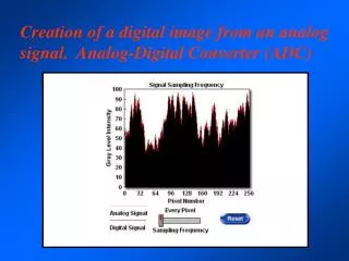
Creation of a digital image from an analog signal. Analog-Digital Converter (ADC)
Creation of a digital image from an analog signal. Analog-Digital Converter (ADC)
Creation of a digital image from an analog signal. Analog-Digital Converter (ADC)
Pixel Saturation: Saturation can be described by the fact that no pixel can be darker than pure black (i.e. value = 0) nor brighter than absolute white (i.e. greater than 255 or 4095 or 65,535)
Pixel Saturation: Once a pixel’s value is saturated it can no longer provide useful information
The data contained in a digital image can be displayed as a histogram which is a plot of the pixel values ranging from black to white versus the number of pixels that have that particular value. Histograms
Low Contrast image (pixels concentrated in a narrow, central values) High Contrast image (many pixels clustered at the extremes of the value range)
Good contrast (even distribution)
One can take an image with a narrow contrast range and expand it to cover the entire range of black to white in a process known as contrast stretching.
The display values of those pixels (i.e. how they will appear on the viewing screen) is determined by the display curve. In the histogram to the left a pixel value of 68 would have a display value of 68. The display curve is straight with a slope of 1.00 Histograms
The slope of the display curve relative to the pixel values can be varied in any number of ways. This is known as a “gamma” correction and can be used to expand the display of either the dark (g < 1) or bright (g >1) portion of the image.
Slope = 1.0 0.5 2.0 Gamma correction can be easily adjusted in many image processing programs by choosing the midpoint of display on the histogram of pixel values and thus changing the slope of the display curve.
Another way of altering the way an image is displayed involves the use of a Look-Up Table or “LUT” in which the value of the input pixel is changed to a new value in the output. Thus a new image matrix is created with new values for each pixel.
This affords much greater control over the displayed image. • Inverted image • All pixels below 100 are black • All pixels between 64 and 120 are black
In applying a color LUT to this image pixels of specific values are displayed as red.
Color LUTs or “CLUT” can be complex and apparently random but if later passed through an inverse CLUT the original image can be restored
Why would having additional bit-depth be important when the human eye can only detect about 100 shades of grey anyhow? X-ray of Breast Contrast Enhanced Subtle differences in grey levels contain information
The fact that digital images are data matrices means that functions can be applied to them. A new data matrix based on the intensity of the pixels in the background can be subtracted from the original matrix and the resultant matrix is then contrast stretched to produce an image in which the distracting background has been substracted.
Dodging and Burning: Selectively increase or decreasing the brightness of a subset of pixels.
Clone Stamp: Selectively copy a portion of the matrix onto another portion of the image.
Clone Stamp: Selectively copy a portion of the matrix onto another portion of the image.
Having increased bit-depth also allows one to take advantage of sophisticated image processing.
Image Processing: Spatial Convolution (image processing) An image processing operation that is used to spatially filter an image. A convolution is defined by a kernel that is a small matrix of fixed numbers. The size of the kernel (3x3, 5x5, 7x7, 9x9) the numbers within it, and a single normalizer value define the operation that is applied to the image. The kernel is applied to the image by placing the kernel over the image to be convolved and sliding it around to center it over every pixel in the original image. At each placement the numbers (pixel values) from the original image are multiplied by the kernel number that is currently aligned above it.
Image Processing: The operation, as defined by the kernel, is applied to all pixels in the original data matrix with the exception of those pixels that form the edge of the matrix. A new output matrix of the same size, but with different pixel values results.
Image Processing: The sum of all these products is tabulated and divided by the kernel's normalizer. This result is placed into the new image at the position of the kernel's center. The kernel is translated to the next pixel position and the process repeats until all image pixels have been processed. As an example, a 3x3 kernel holding all 1's with a normalizer of 9 performs a neighborhood averaging operation. Each pixel in the new image is the average of its 9 neighbors from the original.
Sharpening The sharpness of a digital image refers to the degree of clarity in both coarse and fine specimen detail.
Image processing can be a complex combination of processes First apply apply a color LUT to a greyscale image.
The lowpass averaging filter can be selected from 3x3 up to 255x255 neighborhoods. All pixels included in the filters size are added up, the result is divided by the number of pixels.
The Gauss filter can be selected from 3x3 up to 7x7 kernel size. It performs a weighted sum (center pixel = highest weight). The result is normalized by total kernel weight.
Process / Filters / Median With a kernel size of 3x3 the resulting value is the median (number 5 out of the sorted list of 9). In contrast to lowpass filters, the median keeps edges and removes single pixel errors (like hot pixels) completely.
Laplace (8 connected)The Laplace Filter weights the difference between the center pixel and its neighbors. -1 -1 -1 -1 8 -1 -1 -1 -1
Sharpen (8 connected)Based on the Laplace Filter, the Sharpen Filter includes/adds the original image (center pixels weight one above Laplace) -1 -1 -1 -1 9 -1 -1 -1 -1
SobelThe Sobel filter enhances edges in all directions. It is implemented through two independent convolutions with the left kernel (once rotated by about 90°). The results of each kernel are combined to form the final result. 1 2 1 0 0 0 -1 -2 -1
PrewittThe Prewitt filter performs a similar operation as the Sobel Filter (90° kernel rotate). 1 1 1 0 0 0 -1 -1 -1
The exact sequence of processing steps can bring about a profound change, and improvement, in the image.
The spatial domain is represented by the conventional image. The processes of adjusting contrast, sharpening, background removal, etc. are all forms of spatial convolution. We can also process the data in the image matrix in its frequency domain using algorithms developed by Joseph Fourier Joseph Fourier (1768-1830)
A Fourier Fast Transform (FFT) converts an image into a display of frequencies displayed as an energy spectrum. This can be done optically an an electron diffraction pattern is an example of this, the spacing of dots indicating their frequency and the brightness of the dots indicating the intensity.
A FFT can be created of the spatial domain and if there is a frequency it will show up as dots.
A FFT can be created of the spatial domain and if there is a frequency it will show up as dots. If the size and brightness of the spots is increased the frequency will be enhanced but not changed.