Download
1 / 46
590 likes | 1.06k Views
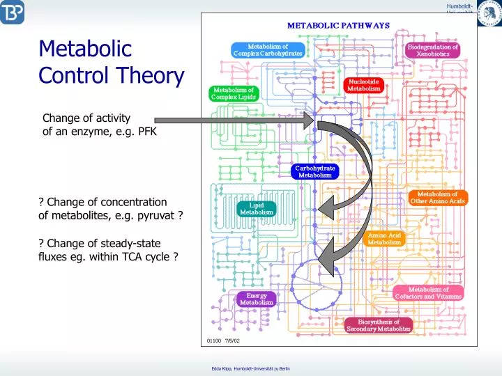
Change of activity of an enzyme, e.g. PFK. ? Change of concentration of metabolites, e.g. pyruvat ?. ? Change of steady-state fluxes eg. within TCA cycle ?. Metabolic Control Theory. Example: Flux Control. Metabolic Control Theory. Quantification of metabolic control

E N D
Change of activity of an enzyme, e.g. PFK ? Change of concentration of metabolites, e.g. pyruvat ? ? Change of steady-state fluxes eg. within TCA cycle ? Metabolic Control Theory
Metabolic Control Theory Quantification of metabolic control Quantification of the impact of small parameter changes on the variables of a metabolic system. Problem: Relations between steady-state variables and parameters are usually non-linear and can not be expressed analytically. There exists no theorie, which permits quantitative prediction of the effect of large changes of enzyme activity on fluxes. Restriction to small (infinitesimal) changes. (Linearisation of the system in vicinity of steady state). Controlling parameters: kinetic constants, enzyme concentrations,... Controlled variables: fluxes, substrate concentrations Wanted: mathematical function quantifying control.
Metabolic Control Theory • Relevant questions: • Many mechanisms and regulatory properties of isolated enzyme reactions are known • what is their quantitative meaning for metabolism in vivo? • Which step of a metabolic systems controls a given flux? • (Is there a rate-limiting step?) • Which effectors or modifiers have the most influence on the reaction rate? • Example: biotechnological production of a substance, Increase of turnover rate • Question: which enzyme to activate in order to yield the most effect? • Example: disease of metabolism, overproduction of a substance • Question: which reaction to modify to reduce overproduction in a predictable way?
Coefficients used in Control Theory Metabolic systems are networks; their behavior depends on the structure of the network and the properties of the individual components. There are two types of coefficients : local and global ones Elasticity coefficients Control coefficients Response coefficients quantify the sensitivity of a rate for the change of a concentration Or a parameter value directly, immediate (no steady state) Quantitative measure for change of steady-state variables Assume reaching new steady states Depends on network structure
Locally: Elasticity Coefficients Question: How sensitive is a rate of an enzyme reaction with respect to small changes of a metabolite concentration? v1 v2 v3 S1 S2 ? ? ? Consider enzyme as isolated, Wanted: immediate effect Elasiticity coefficient of reaction rate k with respect to metabolite concentration Si
Parameter Elasticity -elasticities comprise derivatives with respect to a metabolite concentration (a variable!). -elasticities comprise derivatives with respect to parameter values (kinetic constants, enzyme concentrations,...) v1 v2(Km, Vmax) v3 S1 S2 ?
Globally: Control Coefficients 1. The system of metabolic reactions is in steady state. J = v(S(p),p) S = S(p) 2. A small perturbation of a reaction is performed (Addition of enzyme, addition of metabolite,....) 3. The system approaches a new (nearby) steady state. JJ+DJ SS+DS What is the change of steady state-variables (fluxes, concentrations) due to the perturbation of a single reaction?
Definition of Control Coefficients Flux control coefficient - Change of rate of the k-th reaction under isolated fixed conditions - Resulting change of steady state flux through the j-th reaction - Normalization factor v1 v2 v3 S1 S2 ? ? ?
Definition of Control Coefficients Concentration control coefficient - Change of rate of the k-th reaction under isolated fixed conditions - Resulting change of steady state concentration of Si - Normalization factor v1 v2 v3 S1 S2 ? ?
Choice of Perturbation Parameter The change of vk is based on a change of some parameters pk, which influences only this k-th reaction. (Enzymkonzentration, Inhibitoren, Aktivatoren, ....) Extended expression of flux control coefficient: Important: Perturbation of pk influences directly only vk and no further reaction The flux control coefficients are then independent of the choice of the perturbed parameters pk. The can be interpreted as measure for the degree to which reaction k controls a given flux in steady state.
Response Coefficients, global Consider: complete system in steady state. This state is determined by the values of the parameters; Parameter changes influence the steady state. The sensitivity of steady-state variables with respect to parameter Perturbations is expressed by response coefficients. v1 v2(Km, Vmax, I) v3 S1 S2 ? ? ?
Response Coefficients, Additivity Additivity: If several reactions are sensitive for this parameter v1 v2(p) v3(p) S1 S2 if parameter m influences Only one reaction j :
Example 1 Add inhibitor to a biochemical reaction Experimentelly measurable quantities: Flux control coefficient
Non-normalized Coefficients Non-normalized flux and Concentration control coefficients Non-normalized elasticities Examples Glycolysis: Glucose 2 Lactat Be Control of second reaction? Non-normalized flux control coeff. Normalized coefficients
Theorems of Control Theory The problem: The fluxes J usually cannot be expressed as mathematical functions Of the reaction rates. How can one calculate the global control coefficients from the local (measurable) changes ?? The solution: Use of theoremes. Here, the theoremes are only given and described with examples. The mathematical derivation is given for your information on the following pages.
Thus holds Analog for S1and S2 It follows: The Summation Theorems Thought experiment: What happens, if we induce by experimental manipulation the same fractional change in the local rate of all steps of the system? Result: Flux J must also increase by factor . Since all rates increase in the same ratio, remain the concentration of the variable metabolites S1 and S2 unchanged. The combined effect of all changes in the local rates on the systems variables J, S1 and S2 can be described As the sum of all individual effects caused by the change of each local rate. For flux J holds:
The concentration control coefficients for a substance add up to zero. Some enzymes increase a metabolite concentration, others decrease it. The Summation Theorems The flux control coefficients of a metabolic pathway add up to 1. The enzymes share the control over flux. Matrix notation:
Connectivity Theorems – General Relations Connectivity between flux control coefficients and elasticities Connectivity between concentration control coefficients and elasticities
Example: Calculate flux control coefficients Summation theorem: Connectivity theorem: Result: Since in general: and follows (i.a.!): Both reaction exert positive control over the flux.
Example: Calculate concentration control coefficients Summation theorem: Connectivity theorem: Result: It holds: and Producing reactions have positive control, consuming reactions have negative control.
... v v v v 1 i+1 i r . . . S S S P S P i-1 r - 1 i 1 1 2 Example: Linear pathway S1 S5 S9 Concentration Control Coefficients Reaction Producing reactions have positive control, consuming reactions have negative control.
... v v v v 1 i+1 i r . . . S S S P S P i-1 r - 1 i 1 1 2 Linear Metabolic Pathway Each rate is a function of the concentrations of substrates and productes Assuming mass action kinetics With the equilibrium constants One can derive an equation for the Steady state flux
... v v v v 1 i+1 i r . . . S S S P S P i-1 r - 1 i 1 1 2 Linear Metabolic Pathway – Flux Control General Expression for flux control coefficients (if ) rflux control coefficients 1 summation theorem r-1 connectivity theorems
... v v v v 1 i+1 i r . . . S S S P S P i-1 r - 1 i 1 1 2 Linear Pathway - Properties Ratio of two successive flux control coeff.: Flux control coefficients: Summation theorem Since sum of all flux control coeff is 1, and the ratio of two successive flux control coefficients is positiv, all flux control coefficients in an unbranched pathway are positiv.
... v v v v 1 i+1 i r . . . S S S P S P i-1 r - 1 i 1 1 2 Linear Pathway - Properties Case 1: Be the kinetic constants of all involved enzymes equal and the equilibrium constants larger than 1 Ratio of two successive flux control coeff.: Flux control coefficients tend to be larger at the beginning than at the end.
... v v v v 1 i+1 i r . . . S S S P S P i-1 r - 1 i 1 1 2 Using Relaxation timeas measure for the velocity of an enzyme: All enzymes are involved in control. Slow enzymes exert more control. There is no „rate-limiting step“ Linear Pathway - Properties Case 2: holds: with with or holds and therefore
Flux increase – how? v v v v 3 1 2 4 S S P S P 2 3 1 1 2 Flux control coefficients Simple case: 0.5 0.4 0.3 0.2 0.1 1 2 3 4 Reaction J J + C1 * 1% 1.0053 E1 E1 + 1%
v v v v 3 1 2 4 S S P S P 2 3 1 1 2 v v v v 3 1 2 4 S S P S P 2 3 1 1 2 v v v v 3 1 2 4 S S P S P 2 3 1 1 2 Flux increase v v v v 3 1 2 4 S S P S P 2 3 1 1 2
Irreversibility and Feedback v 3 v v 1 2 v 4 S S P S P 2 3 1 1 2 v 3 v v 1 2 v 4 S S P S P 2 3 1 1 2 v 3 v v 1 2 v 4 S S P S P 2 3 1 1 2
Branching System v1 v2 v3 P0 S1 S2 P3 v4 v5 P4 P5
P v 2 2 ATP v ADP 1 S P ATP 1 ADP v 3 P 3 G 0 Branching Systemwith ATP/ADP-Exchange Rang(N) = 2 < r Conservation relation ATP + ADP = const. Reduced stoichiometric matrix Basis vector for admissible steady state fluxes
Mathematical Derivation of the Theorems Start with equation Implicite Differentiation w.r.t. parameter vector p regular Jacobi matrix M Rearrange to Rearrange to
Mathematical Derivation of Theorems, 2 Start with equation Implicite differentiation w.r.t. parameter vector p Non-normalized Flux CC Rearrange to Both non-normalized CC are independent of the choice of perturbed parameter. They depend only on stoichiometry (N) and kinetics (dv/dS) !!
Reaction System with Conservation Relations Problem: Jacobi-Matrix is not regular Rearrange rows of N and S, Such that dependent rows are at bottom. Implicite Differentiation of independent steady-state equations w.r.t parameter vector p The non-singular Jacobi matrix Of the reduced systems : Non-normalized concentrations cc Non-normalized flux cc
Glcx Glc G6P F6P FBP GAP DHAP BGP PEP Pyr ACA EtOH EtOHx Glyc Glycx ACAx CNx ATP ADP NAD+ NADH AMP 1 2 3 4 5 6 7 8 9 10 11 12 13 14 15 16 17 18 19 20 21 22 23 24 Real System – GlycolysisConcentration control coefficients
Concentration control in the MAP K cascade 3 1 MAPKKK MAPKKK-P MAPKKK-PP 4 2 5 7 MAPKK MAPKK-P MAPKK-PP 8 6 11 MAPK 9 MAPK-P MAPK-PP 12 10 All parameter values: k, p=1
v2 v1 S1 v3 S2 S4 v4 S3 v5 Non-Steady State Trajectories S1 S1[0] = 0 S2[0] = 0 S3[0] = 0 S4[0] = 1 What is the effect of parameter perturbations on time courses ? S2 S[t] S4 S3 p1 p2 p1 = 1 p2 = 1 p3 = 1 p4 = 0.5 p5 = 0.5 S2[0] S4[0] S1[0] p3 p1,3 RS2 S3[0] p5 p4 p2 p4 p5 p5 S3[0] RS3 S4[0] p1,3 S2[0] S1[0] p2 B.P. Ingalls, H.M. Sauro, JTB, 222 (2003) 23–36 p4 Time
Time-dependent Response: B.P. Ingalls, H.M. Sauro, JTB, 222 (2003) 23–36
Experimental Methods to Determine Control Coefficients - Titration with purified enzyme - Addition of specific inhibitors - Overexpression of an enzyme using genetic techniques - Downregulation of individual genes / Reduction of enzyme amount
Metabolic Control Analysis - History/People 1973 Kacser /Burns 1974 Heinrich /Rapoport - Definition of coefficients about 1980 Discovery by Experimentalists (Westerhoff) 1988 Reder – Matrix Formulation BTK - Models and Experiments (Fell, Cornish-Bowden, Hofmeyr, Bakker, Schuster,….)