Download

1 / 12
160 likes | 537 Views
Normal Distributions and the Empirical Rule. Learning Target: I can use percentiles and the Empirical rule to determine relative standing of data on the standard normal curve. 2.2 a Hw: pg 131: 42, 44, 45, 50, 51. Normal distributions: N ( μ, σ). Symmetric , single peaked and bell shaped.

E N D
Normal Distributions and the Empirical Rule Learning Target: I can use percentiles and the Empirical rule to determine relative standing of data on the standard normal curve. 2.2 a Hw: pg 131: 42, 44, 45, 50, 51
Normal distributions: N (μ, σ) • Symmetric, single peaked and bell shaped. • Center of the curve are μ and M. • Standard deviation σ controls the spread of the curve.
Normal distributions: N (μ, σ) • Inflection points: points where change of curvature takes place is located a distance σ on either side of μ.
Normal curves are a good description of some real data: • test scores • biological measurements • also approximate chance outcomes like tossing coins
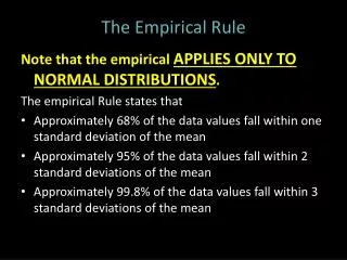
The Empirical rule (68-95-99.7 rule) In the normal dist. with mean μ and standard deviation σ. • 68% of the observations fall within of the mean. • 95% of the observations fall within of the mean. • 99.7% of the observations fall within of the mean. 1σ 2σ 3σ
Percentiles:we are interested in seeing where an individual falls relative to the other individuals in the distribution. • First quartile – 25th percentile • Median – 50th percentile • Third quartile – 75th percentile
Ex. 1: Percentiles 84% tile Find the percentiles on above graph at 1, 2 and 3σ’s above and below μ. • At 1σ: 1 - .68 = .32 • 0.32 lie shared above and below 1σ so,.32/2 = .16 • At 1σ above the mean; • 1 – 0.16 = 0.84
Percentiles 84% tile 97.5th % 99.85th % • At 2σ above the mean; • 1 – .025 = 0.975 • At 3σ above the mean; • 1 – 0.0015 = 0.9985
84% tile 16%tile 97.5th % 2.5%tile .15%tile 99.85th % • Use similar method to find percentiles below the mean • At σ below the mean • At 2σ below the mean • At 3σ below the mean
Exercise 2: Men’s Heights The distribution of adult American men is approximately normal with mean 69inches and standard deviation 2.5 inches. Draw the curve and mark points if inflection.
Recall: mean 69 in. and standard deviation 2.5 in. 16%tile 84% tile 2.5%tile 97.5th % 2.5% .15%tile 99.85th % 64 74 61.5 64 66.5 69 71.5 74 76.5 a) What percent of men are taller than 74 inches? 74 is two standard dev. above the mean. 2.5% b) Between what heights do the middle 95% of men fall? 69 5 =
mean 69 in. and standard deviation 2.5 in. 16% 84% 61.5 64 66.5 69 71.5 74 76.5 c) What percent of men are shorter than 66.5 inches? 16% d) A height of 71.5 inches corresponds to what percentile? 1 - .68 = .32 .32/2 = .16 1 - .16 = .84