Download
1 / 122
1.81k likes | 2.83k Views
Chapter 1 = Systems of Linear Equations & Matrices. MATH 264 Linear Algebra. Introduction.

E N D
Chapter 1 = Systems of Linear Equations & Matrices MATH 264 Linear Algebra
Introduction • Information in science, business, and mathematics is often organized into rows and columns to form rectangular arrays called “matrices” (plural of “matrix”). Matrices often appear as tables of numerical data that arise from physical observations, but they occur in various mathematical contexts as well. • Example:
Linear Equations • A line in a 2D plane (or x-y coordinate system) can be represented as • And a line in a 3D plane as • The following are examples of linear equations • The following are NOT linear equations
A finite set of linear equations are called linear systems (or systems of linear equations) • The variables are our unknowns • A general linear system of m equations in the n unknowns are written as
2 & 3 Unknowns in Linear Systems • Linear systems in two unknowns arise in connection with intersections of lines. For example, consider the linear system in which the graphs of the equations are lines in the xy-plane. Each solution (x, y) of this system corresponds to a point of intersection of the lines, so there are three possibilities
In general we say that the linear system is consistent if it has 1 solution • No solutions means the linear system is inconsistent
Augmented Matrices • As the number of equations and unknowns increase, so does the complexity of solving the system of linear equations. • We can abbreviate the linear system by • partitioned matrix augmented matrix
What are Augmented Matrices? • An augmented matrix of a system of linear equations is really just that system without the variables and signs (+ - x / =) • The augmented matrix for
Elementary Row Operations • The basic method for solving a linear system is to perform appropriate algebraic operations on the system that do not alter the solution set • The 3 common row operations performed on a matrix: • Multiply a row through by a nonzero constant • Switch two distinct rows • Add one row to another row
Gaussian Elimination,Row Echelon Form (REF), Gauss-Jordan Elimination, and Row Reduced Echelon Form (RREF)
Introduction to Elimination • In this section we will develop a systematic procedure for solving systems of linear equations. • The procedure is based on the idea of performing operations on rows of augmented matrix that simplify it to a form from which the solution to that system can be found. • Almost all of the methods that are used for solving large systems of equations are based on the simple laws that we will develop here.
Reduced Row Echelon Form (RREF) To be RREF a matrix must have: • If a row does not consist entirely of zeros then the first nonzero number in the row is a 1. • If there are any rows that consist entirely of zeros then they are grouped together @ bottom of matrix • In any 2 successive rows that do not consist entirely of zeros the leading 1 in the lower row occurs farther to the right than the leading 1 in the higher row • Each column that contains a leading 1 has zeros everywhere else in that column
A matrix that has the first 3 properties is in ROW ECHELON FORM. • A matrix that has all 4 properties is in REDUCED ROW ECHELON FORM.
Definitions • General Solution = A set of parametric equations from which all solutions can be obtained by assigning numerical values to the parameters. Applicable only when a linear system has many solutions. • An m X n matrix is a rectangular array of numbers with m rows and n columns • Size and arrangement matters
The 3 Elementary Row Operations • Scale a row by a non-zero real number • Add a non-zero multiple of one row to another • Exchange two rows Example of how to do this is shown on next slide
Just keep doing Steps 1 – 4 for all the other rows… Note: some steps are missing and the final result is shown below
Determining solutions from REF of augmented matrix • We use Gaussian elimination to put the augmented matrix of a system of linear equations in REF (row echelon form). • If the augmented matrix of a system is in row echelon form, we can determine the solutions using substitution, starting with the last equation and working upward. This is method of back-substitution
Possibilities for solutions • The system has no solution = therefore the system is inconsistent • The system has a unique solution = therefore the system is consistent • The system has infinitely many solutions THEOREM: If a REF of the augmented matrix of a system of equations has a leading 1 in the final column then the system is inconsistent & has no solutions.
More on the Theorem • If the row echelon form of the augmented matrix of a system of linear equations does not have a leading 1 in the final column then the system has asolution.