Download
1 / 61
610 likes | 701 Views
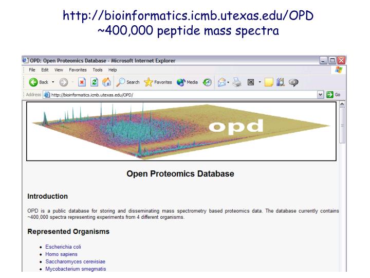
http://bioinformatics.icmb.utexas.edu/OPD ~400,000 peptide mass spectra. A few diverse examples of proteins:. A muscle protein:. aspirin. A virus protein shell (“capsid”):. Watercolors by David Goodsell, Scripps. Outline. Part I What dictates the 3D shape (“fold”) of proteins?

E N D
http://bioinformatics.icmb.utexas.edu/OPD ~400,000 peptide mass spectra
A few diverse examples of proteins: A muscle protein: aspirin A virus protein shell (“capsid”): Watercolors by David Goodsell, Scripps
Outline Part I What dictates the 3D shape (“fold”) of proteins? 1. Primary structure of proteins - amino acids & peptide bonds 2. Secondary structure of proteins - “local” folding topology & predicting 2° structure 3. Tertiary structure of proteins - “global” folding topology - X-ray crystallography & NMR - aligning structure computationally - protein folding - designing new structures Part II How do proteins interact with each other in the cell?
solvent accessible surface “ribbon” = Ca backbone Different representations of a typical globular protein (myoglobin) ribbon + stick-figure side chains all atoms drawn at van der waals radii
Due to resonance forms of the peptide bond: Peptide bonds (N-CO) are planar, so only allowed rotation along amino acid backbone is around Ca-N and Ca-CO bonds ==> by convention angles called F & Y Protein folding = the selection of F/Y angles & side chain angles leading to low energy packing of the atoms
A Ramachandran plot shows only certain F/Y combinations are sampled, dictated by steric hindrance of atoms neighboring peptide bond Favored regions correspond to secondary structures ==> allowable “local” structural conformations
3 of the most common secondary structures a helix 3.6 aa’s/turn http://www.rtc.riken.go.jp/jouhou/image/protein/2ndst/2ndst.html
Amino acids vary in their intrinsic propensities to adopt the different secondary structures
Given aa sequence, how to predict 2° structure? ==> PhD input = 13 aa sliding window - neural network, predicts 3 states: a helix, b strand, coil & relative level of solvent accessibility ==> 3 state prediction accuracy ~72% http://maple.bioc.columbia.edu/predictprotein/
A 0.4 B 0.1 C 0.3 ... ... emission probabilities Hidden states transition probabilities A 0.1 B 0.3 C 0.4 ... ... emission probabilities Some proteins have unusual secondary structures that span membrane => membrane proteins How to identify transmembrane segments in a protein? Current best approach, TMHMM is based on Hidden Markov models. Y A generic HMM: X Hidden state seq: Observable seq: XXXXYYYYXXXY CCBCCAAABCAC Goal = recover hidden state sequence by analyzing emissions
TMHMM hidden Markov model inside & outside loop models, helix cap models HMM for 5-25 aa helix core Correctly predicts >90 % of the transmembrane helices Discriminates between soluble and membrane proteins with false positive rate ~1% Krogh et al, J Mol Biol. 305:567-80 (2001)
Packing of secondary structures leads to more complex 3D assemblies (“motifs”):
Tertiary structure = 3D packing of secondary structural elements - Hydrophobic residues (Phe, Ile, Leu, Trp) buried in the core - Core densely packed; not room even for H2O, comparable to a typical crystal - Core atoms so close that van der Waals bonds contribute significantly - Charged and polar R groups (e.g., Arg, Lys, Glu, Asp, His) on outside and hydrated
Experimental approaches to protein structure I X-ray crystallography crystal of pure protein Rotate crystal, collect amplitudes of diffracted X-rays as function of incident angle of X-rays Find phases of diffracted X-rays (by experiment or computation) With phases & amplitudes, Fourier transform to find distribution of electrons (“electron density”) in protein Electrons in crystal diffract X-rays according to Bragg’s Law: nl = 2d sinq wavelength angle of X-rays to plane of atoms distance between atomic layers in crystal Build atomic model into electron density, refine From B. Rupp’s X-ray crystallography intro: http://www-structure.llnl.gov/Xray/101index.html
Experimental approaches to protein structure II Nuclear magnetic resonance protein in solution in center Vary radio wave pulses, Measure field generated in response over time => function of chemical environment of each nucleus Assign identities to nuclei, measure distances between amino acid atoms Use distance geometry to solve for ensemble of 3D structures consistent with distance constraints very strong magnet coils to send/detect radio waves Basic principle: Atomic nuclei w/ odd mass #’s have spin ==> charged, spinning particles & produce magnetic field In an external magnetic field, this nuclear magnetic field precesses around an axis Can observe this process by applying radio wave pulses at frequencies related to precession frequencies & measuring the resulting induced electric current Flemming Poulson, A Brief Introduction to NMR spectroscopy of proteins.
3 broadest classes of protein 3D structures Fibrous e.g., collagen Membrane e.g, K+ channel & Globular ...
Examples of globular protein “folds” all a a/b all b a+b
>24,000 experimentally determined protein structures stored in PDB database: http://www.rcsb.org/pdb/
Atomic coordinates of a protein structure (PDB format) - first 3 aa’s = Met-Glu-Ala... atomic coordinates occupancy aa type & # atom type x y z atom # & name B-factor ATOM 1 N MET A 1 32.632 -11.712 53.840 1.00 63.20 N ATOM 2 CA MET A 1 31.203 -12.125 53.853 1.00 63.20 C ATOM 3 C MET A 1 30.947 -12.743 55.207 1.00 63.20 C ATOM 4 O MET A 1 31.741 -13.533 55.685 1.00 63.20 O ATOM 5 CB MET A 1 30.931 -13.144 52.733 1.00 96.70 C ATOM 6 CG MET A 1 29.500 -13.132 52.189 1.00 96.70 C ATOM 7 SD MET A 1 28.784 -14.774 52.145 1.00 96.70 S ATOM 8 CE MET A 1 27.934 -14.832 53.770 1.00 96.70 C ATOM 9 N GLU A 2 29.841 -12.367 55.822 1.00 61.59 N ATOM 10 CA GLU A 2 29.498 -12.881 57.128 1.00 61.59 C ATOM 11 C GLU A 2 28.134 -12.349 57.527 1.00 61.59 C ATOM 12 O GLU A 2 28.043 -11.213 57.995 1.00 61.59 O ATOM 13 CB GLU A 2 30.533 -12.408 58.152 1.00 51.85 C ATOM 14 CG GLU A 2 30.050 -12.440 59.600 1.00 51.85 C ATOM 15 CD GLU A 2 30.843 -11.520 60.513 1.00 51.85 C ATOM 16 OE1 GLU A 2 31.432 -10.532 60.018 1.00 51.85 O ATOM 17 OE2 GLU A 2 30.858 -11.780 61.737 1.00 51.85 O ATOM 18 N ALA A 3 27.077 -13.140 57.353 1.00 71.14 N ATOM 19 CA ALA A 3 25.751 -12.666 57.749 1.00 71.14 C ATOM 20 C ALA A 3 25.735 -12.594 59.298 1.00 71.14 C ATOM 21 O ALA A 3 25.475 -13.591 59.986 1.00 71.14 O ATOM 22 CB ALA A 3 24.678 -13.608 57.214 1.00 34.69 C
Some of the major computational questions in structural biology 1. How to distinguish membrane proteins from soluble proteins ? 2. How to align protein structures & start organizing them into families, etc. ? 3. How to predict folded protein structure from the linear amino acid sequence? 4. How to identify the active/functional region of the protein from the structure? 5. How to predict the interactions of drugs or other proteins from the structure? 6. How to computationally predict the structural consequences of mutations? 7. How to predict protein function from structure? 8. How to design new or unnatural protein structures?
How to find the best superposition of 2 protein structures? Note: superimposing 2 structures is easy if you know the equivalent amino acids -> the hard part is to find this mapping of atoms from 1 structure to the other One now-classic approach: DALI Align sequence #1 to sequence #2 so as to maximize similarity in contact patterns Amino acid # Amino acid # Protein #1 structure Ca coordinates only Calculate matrix of all pairwise Ca-Ca distances Repeat for protein # 2 Holm & Sander, J Mol Biol. 233:123-38 (1993)
Best structural alignment corresponds to maximizing i, j = aligned pairs of matched residues i = iA, iB j=jA,jB f = similarity of 2 Ca-Ca distance matrices, dAij and dBij In the simplest case, where dAij and dBij are equivalenced residues in proteins A and B. and q R = minimum level of similarity Choose mapping of residues (e.g. iA to iB) to minimize dAij- dBij iA iB dAij dBij jA jB Protein A Protein B
The ability to compare structures has led to recognition of a hierarchy of 3° structures (“folds”) Class As organized in the CATH or SCOP or FSSP databases: Architecture Manual classification at architecture level, automated at topology level Topology Homologous Superfamily H flavodoxin homologues
Protein Folding Classic experiment from 1960’s (Chris Anfinsen): Purified small protein RNaseA, Refolded in a few minutes in solution ==> all information necessary for correct folding was captured in the linear amino acids sequence Corollary: Proteins do not fold by randomly testing conformations. Given a 100 amino acid protein, & 10 possible conformations / amino acids = 10100 possible conformations for the protein ==> not possible to randomly sample, clearly constrained search
An energetic view of the folding process Fast Slow Large # of conformationally different molecules Collection of similar conformations interconverting Unique or small # of final conformations optimize packing T “hydrophobic collapse” U free energy M F Molten globule Transition state Unfolded Folded folding trajectory Local secondary structures form first Adapted from Branden & Tooze
One long-time goal of biologists/biophysicists: Solvethe Protein Folding Problem = computationally predict protein 3D fold from 1D amino acid sequence Two general approaches: 1st principles/ab initio: e.g., atomistic molecular dynamics simulations of proteins, modeling force fields w/ electrostatic, van der waals forces, solvent, etc. over long time Empirical: - fold recognition/threading - reverses the process: given set of structures, learn empirical rules that predict folds Empirical currently more successful at predicting final structure, but no information about folding trajectory
An example of a successful design of a new protein fold by a combination of empirical & ab initio structural modeling designed 93 amino acid protein with topology not in PDB dbase designed model solved structure Kuhlman et al, Science, 302:1364-1368 (2003)
The Kuhlman et al. design strategy Starting model = Choose predefined 3D topology Assemble 3D model from 3 and 9 amino acid fragments of known structure ==> Generated 172 backbone-only starting models Initialization Choose optimal sequence for each starting model using energy function that captures: 12-6 Lennard-Jones potential orientation-dependent hydrogen bonding term implicit solvation model Choose amino acid side chain orientations (“rotamers”) by sampling from known structures Iterate between: Optimize choice of amino acid sequence for a fixed backbone conformation Optimize amino acid backbone coordinates for a fixed sequence Same energy function used at all stages Only previous lowest energy sequence/structure optimized at each stage Final designed sequence not similar to any known protein sequence Kuhlman et al, Science, 302:1364-1368 (2003)
References A good introduction to structural biology = Introduction to Protein Structure - Carl Branden & John Tooze Web resources: Protein Data Bank = > 24,000 protein structures, atomic coordinates, & the “protein of the month” http://www.rcsb.org/pdb CATH/SCOP protein structure hierarchies: http://www.biochem.ucl.ac.uk/bsm/cath/ http://scop.mrc-lmb.cam.ac.uk/scop/ Several of the illustrations in this tutorial were taken from Lehninger Principles of Biochemistry, by Nelson & Cox
Macrophage (“white blood cell”) Blood serum Bacterium “Macrophage and Bacterium 2,000,000X” Watercolor by David S. Goodsell, 2002
Typical size ranges of known protein structures & assemblies single protein domain dimeric protein aquaporin (membrane channel) Ribosome From a (recommended) review article==>Sali et al. Nature 422:216-225 (2003)
Outline Part I What dictates the 3D shape (“fold”) of proteins? Part II How do proteins interact with each other in the cell? 4. “Quaternary” structure of proteins & protein interactions 5. Experimental approaches to determine interactions - yeast 2 hybrid, mass spectrometry 6. Testing the accuracy of the interactions 7. Moving back to the atomic resolution world - electron microscopy & tomography - modeling structures of complexes
Why study interactions? Proteins interact all the time (e.g., bump into each other non-specifically) We’re interested in specific interactions ==> e.g., those w/ downstream consequences For example, consequences might include: Inducing a change in the structure of an interaction partner Stabilizing or destabilizing an interaction partner Modifying the activity of a protein (activate, inhibit, or otherwise regulate) Cause interaction partner to move to another location Cut interaction partner Chemically modify interaction partner (phosphorylate, dephosphorylate, glycosylate, deglycosylate, ubiquitinate, sumoylate, etc... ==> more than 200 modifications to proteins known, many catalyzed by other proteins So, defining interactions helps to define these processes & their functional consequences
Experimental/Computational methods for observing/inferring protein interactions Sali et al. Nature 422:216-225 (2003)
X-ray structure of ATP synthase Schematic version Network representation a b g d b2 e a c12 Total set = protein complex Sum of direct + indirect interactions
Some methods measure direct interactions, some indirect Xenarios & Eisenberg, Curr. Op. Biotech. 12:334-9 (2001)
Interactions between yeast proteins
Experimental approaches to protein interactions I Yeast two-hybrid Prey Act DBD Bait + DBD “Bait” “Prey” Act DNA binding domain Transcription activation domain Core transcription machinery transcription operator or upstream activating sequence Reporter gene Basic idea = screen library of “prey” proteins to test which ones interact with a given “bait” protein Fields & Song, Nature 340:245-6 (1989)
Experimental approaches to protein interactions I High-throughput yeast two-hybrid I Haploid yeast cells expressing activation domain- prey fusion proteins Diploid yeast probed with DNA-binding domain- Pcf11 bait fusion protein Uetz et al. Nature 403 (2000)
A second group (Ito et al.), with a related yeast two-hybrid approach, also mapped a large number of interactions, then compared the interactions w/ the Uetz data: A surprise at the time was the apparent inconsistency among the interaction sets ==> either # of potential interactions is large or false positive rate high (or both) Ito et al. PNAS 98:4569-74 (2001)
Experimental approaches to protein interactions II Mapping complexes by mass spectrometry I “Bait” protein Interaction partners co-purified with “bait” Tag 493 bait proteins 3617 “interactions” Affinity column protein 1 protein 2 Ho et al. Nature 415 (2002) protein 3 SDS- page Trypsin digest, identify peptides by mass spectrometry protein 4 protein 5 protein 6
Experimental approaches to protein interactions I A variant: Tandem affinity purification (TAP) + Mass spectrometry Tag1 Tag2 Bait Affinity column2 protein 1 protein 2 Affinity column1 protein 3 SDS- page protein 4 protein 5 + protease protein 6 Trypsin digest, identify peptides by mass spectrometry Affinity column1 Rigout et al., Nature Biotech. 17:1030-2 (1999)
How accurate are these high-throughput screens? Can compare to known interactions, but these are incomplete A different strategy is to identify properties that correlate with interactions & test versus those properties Three tests: 1. Comparison of interactions to a reference interaction set 2. Comparison of mRNA co-expression of interacting partners 3. Comparison of functions of predicted interaction partners
Estimate accuracy by comparing to a well-determined reference set of interactions Test #1 (tends to underestimate accuracy) von Mering, Krause et al. Nature May 8, 2002
Estimating interaction assay accuracy by assessing mRNA co-expression of putative interaction partners Random Protein Pairs True interactions Correlation coefficient between expression vectors derived from many DNA microarray experiments Test #2 Estimate % false positives from observed vs. expected genes w/ correlated expression Estimated false positive rates based on this test: Mrowka et al. Genome Research 11:1971-3 (2001)
A related strategy: fit distribution of co-expression relationships as mix of those from random & well-characterized interactions ==> Mixture % indicates accuracy. Deane, Salwinski et al. Mol. Cell. Proteomics (2002)