Download
1 / 29
290 likes | 296 Views
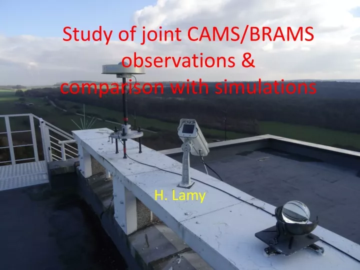
Study of joint CAMS/BRAMS observations & comparison with simulations. H. Lamy. Forward scatter radio observations. 2 advantages : Continuous monitoring Sensitive to smaller masses. Duration of the meteor echo depends roughly on the size of the object

E N D
Study of joint CAMS/BRAMS observations &comparison with simulations H. Lamy
Forwardscatter radio observations • 2 advantages: • Continuous monitoring • Sensitive to smaller masses • Duration of the meteorechodependsroughly on the size of the object • Most meteorechoes last a fraction of a second.
The BRAMS network • 49.97 MHz • 150 W • pure sine wave • circularly polarized
The BRAMS network University of Mons Maasmechelen Uccle Neufchâteau
Example of BRAMS data 3 MB per file every 5 min 1 GB of data per day and per station WAV-format
Spectrograms 200 Hz 5 minutes NFFT = 16384 – overlap = 90% t 0,34 sec (real 2,97 sec) and f 0,3 Hz
General idea • We are still struggling with the algorithms to retrieve meteoroid trajectories from BRAMS multi-stations observations. • Meanwhile we propose to use CAMS observations above Belgium which provide very accurate trajectories and speeds
CAMS observations Credit : P. Roggemans Provide very accurate trajectories, speed and deceleration measurements Jenniskens et al (2016)
CAMS observations • Night from 19 to 20 January : 245 trajectories • Trajectory 240 : • V_ = 66.33 0.15 km/s • a1 = 0.017 0.01 km/s • a2 = 0.398 0.08 s-1 • Lat, Long, H of begin and end points of CAMS trajectory • Begin time of observation of CAMS trajectory
Red : CAMS visual trajectory CAMS t_begin CAMS t_end Tx Rx1 Rx2 Rx3
CAMS/BRAMS 1st comparison Night from 19 to 20/01/2017 : 245 trajectories Trajectory 240 Not all stations were working nominally !
CAMS/BRAMS 1st comparison Zt =102.3 km Zt =93.1 km
CAMS/BRAMS 1st comparison Zt = 117.4 km Zt = 120.5 km
Amplitude (a.u.) Time (sec) Blackman filter
CAMS/BRAMS more accuratecomparison Check that the time corresponding to (e.g.) Half Maximum Power is close to the theoretical time due to specular reflection
Determination of peak power Ppeak-under = Mc Kinley (1961)
Gains of the Tx / Rxantennas GR(,) Credit : A. Martinez Picar
Calibration of peak power « Calibrated » value by determining the amplitude of the calibrator signal Ppeak-under in Watts
Limitations • Mc Kinley’s formula is strictly valid for underdense meteor echoes. Quid for overdense ones or even those with intermediate electron line densities? • Most antennas were tilted at that time, which means that their gain GR(,) is not very well constrained in the direction to the reflection point. • For the polarisation factor, we can tentatively take ½ (assuming we emit a circularly polarised wave, which is not exactly the case) • We have also to check the stability of the calibrator over time • Not all stations were working nominally at that time (problems with receiver, no calibrator everywhere, mismatch of antennas, etc…)
Electron line densities We obtain the linear electron line density in different points along the meteoroid path
Comparisonwith simulations First, with a relatively simple model such as the one from Vondrak et al (2008). Matlab code available from VKI • V and given by CAMS • massumedwithtypical values (unlessother information available) • Onlyunknownremains the mass
Comparisonwith simulations q is the ionisation rate (in e-/m3) General idea : • Run the model for several « reasonable » values of the initial mass. Each model produces a profile of q as a function of the distance along the meteoroid path • Pick up the value of the mass that minimizes (in least square sense) the difference between simulated values and values obtained from BRAMS data • For that, establish link between q and
Perspectives • Correct the existing codes to analyze BRAMS/CAMS data and make them robust • Run the Matlab codes for the Vondrak model and pick up the best solution • Use more recent data from 4/5 October 2018 – 522 orbits • Present these results at EGU meeting – Vienna – 7-12 April 2019 • Publish the results • Explore other possibilites to decrease the aforementioned limitations