Download
1 / 106
1.1k likes | 1.44k Views
Stochastic Geometry as a tool for the modeling of telecommunication networks. Prof. Daniel Kofman, ENST - Telecom Paris Dr. Anthony Busson IEF – University of Orsay-Paris 11. TAU – 25/11/2004. S.G. and Network Modeling.

E N D
Stochastic Geometry as a tool for the modeling of telecommunication networks Prof. Daniel Kofman, ENST - Telecom Paris Dr. Anthony Busson IEF – University of Orsay-Paris 11 TAU – 25/11/2004
S.G. and Network Modeling • When modeling a network, two main types of characteristics need to be captured: • the dynamics imposed by the traffic evolution at different time scales • time properties • the spatial distribution and movement of network elements (terminals, antennas, routers, etc.) • geometric properties
Examples of Geometric Properties • Modeling of • UMTS/WiFi antennas location • optimal cost under coverage constraints • Sensor networks • optimal cost under coverage, connectivity and lifetime constraints • Ad-Hoc Networks • CDN servers location for optimal content distribution • Multicast capable routers of a CBT architecture • Reliable Multicast Servers for optimal retransmission of missed information • Networks Interconnection points • Optimal placement of fix access networks concentrators • Others
Why Stochastic Geometry • The efficiency of a protocol/mechanism/ dimensioning rule, etc. depends on its adaptability to different network topologies and users distribution • The performance metrics of interest have usually to be obtained as an average over • A large set of possible network topologies • A large set of possible users location distribution • Members of the various multicast groups • Clients of the different available content • A large set of users behaviors • Mobility • Content popularity
Content • Introduction • Application domains in the telecommunication world • Why Stochastic Geometry (S.G.)? • A Simple example to illustrate what S.G. is • Network infrastructure optimization • Theoretical framework, part 1 – Tessellation processes • Other application examples (CDNs, Multicast routing) • Theoretical framework, part 2 – Coverage processes • More application examples (CDMA, Ad-hoc and sensor networks) • Summary: Main mathematical objects, Main known results • Conclusions and Perspectives
Content • Introduction • Application domains in the telecommunication world • Why Stochastic Geometry (S.G.)? • A Simple example to illustrate what S.G. is • Network infrastructure optimization • Theoretical framework, part 1 – Tessellation processes • Other application examples (CDNs, Multicast routing) • Theoretical framework, part 2 – Coverage processes • More application examples (CDMA, Ad-hoc and sensor networks) • Summary: Main mathematical objects, Main known results • Conclusions and Perspectives
A simple example: Network infrastructure optimization • Network topology to be modeled: • Users are connected to the closest Service Provider Point of Presence (PoP) • PoP are hierarchically connected to the closest concentrator • Higher layer concentrators are connected to the closest core equipment • Core equipment are “meshed”
Architecture PoP Core Conc. PoP Access Network
Questions we can answer • For a given distribution of users and for a given cost function, under Poisson hypothesis, we can compute the • Optimal number of hierarchical levels • Optimal intensity of the various point processes • Average number of users per PoP • Average cost of the network • Routing cost in number of hops when connection two clients as a function of their distance • For the detailed analysis of this model see • F. Baccelli, M. Klein, M. Lebourges, and S. Zuyev. Stochastic geometry and architecture of communication networks. J. Telecommunication Systems, 7:209-227, 1997.
Content • Introduction • Application domains in the telecommunication world • Why Stochastic Geometry (S.G.)? • A Simple example to illustrate what S.G. is • Network infrastructure optimization • Theoretical framework, part 1 – Tessellation processes • Other application examples (CDNs, Multicast routing) • Theoretical framework, part 2 – Coverage processes • More application examples (CDMA, Ad-hoc and sensor networks) • Summary: Main mathematical objects, Main known results • Conclusions and Perspectives
Stationary Poisson point process in d • Definition • The number of points in a set B of d follows a discrete Poisson law of parameter l.||B||, where l is the intensity of the process • Let B1…Bn be disjoint sets of d, the number of points in B1 … B2 are independent. • Consequence • Given n the number of points in B, the points are independently and uniformly distributed in B.
Poisson Voronoï tessellation • The point process generating the Voronoï tessellation is a stationary Poisson point process. • The mathematical theory is studied by Møller • See [Møller 89,94] • Main characteristics • λ : pp intensity • λ0 =2λ (vertices intensity)
Poisson Voronoï Tessellation • The point process generating the Voronoï tessellation is a stationary Poisson point process. • The mathematical theory is studied by Møller [Møller] • Main characteristics • l : pp intensity • l0 =2l • l1 =3l (sides intensity)
Characteristic of the « typical cell » • Number of sides (6 in average) • Area (1/ l in average) • Average perimeter length :
Expectation under Palm measure Cost function • A point at x add a cost f(x,N). • In this case, the mean of the cost function is: • By the refined Campbell formula, we have:
Palm measure: intuitive introduction D(1)/D(0,8) 1 Number of packets 0,8 D D 1 Arrival U(1) Departure 0 time Prob (Queue empty)=0,2 Prob (Queue empty at arrival times)=1 Prob0(Queue empty)=1 PASTA: Poisson Arrivals See Time Averages
Feller’s Paradox for a Poisson Process • Bus inter-arrival process: Poisson of parameter l • Bus inter-arrival times sequence: i.i.d., exp(l) • Waiting time for a passenger arriving at time t: exp(l) • Time since last bus arrival before time t: exp(l) • Probability distribution of the inter-arrival containing time t: Erlan-2 of parameter l • Average inter-arrival time 1/ l • Average length of the inter-arrival containing time t: 2/ l t time
Feller’s paradox and Palm theory • Since we look at stationary processes, time t could be whatever. • We will concentrate without loss of generality in the case t=0. • By definition of Palm probability (at time 0), we have • Prob0(T0=0) = 1 • The inter-arrival time sequence is i.i.d., exp(l) • Since the intervals generated by each point of the process are equivalent, we can concentrate in any of them, like the one starting at 0, when analyzing the performances of the system.
Plane case E(C0()) = / with =1.280 E0(C0()) = 1/
Expectation under Palm measure Back to Campbell Formula • A point at x add a cost f(x,N). • In this case, the mean of the cost function is: • By the refined Campbell formula, we have:
Summary • The location of the various elements is modeled by point processes • Voronoï Tessellations are used to partitioning the plane and deducing the elements connectivity • Delaunay graph/tessellations can be used for the same purposes • A cost function is defined as a functional of the previous processes • Palm theory is used to evaluate this cost function we want to optimize
Content • Introduction • Application domains in the telecommunication world • Why Stochastic Geometry (S.G.)? • A Simple example to illustrate what S.G. is • Network infrastructure optimization • Theoretical framework, part 1 – Tessellation processes • Other application examples (CDNs, Multicast routing) • Theoretical framework, part 2 – Coverage processes • More application examples (CDMA, Ad-hoc and sensor networks) • Summary: Main mathematical objects, Main known results • Conclusions and Perspectives
Internet Example 2: Content Distribution User Content Provider Server
Content Delivery Network • Problems : • The provided QoS depends on the network performances • Thus, the content provider cannot control this quality • The content on the cash servers cannot be controlled • Solution : • To deploy a set of servers • Expensive • To share the resources of a CDN between various Content Providers
Internet What is the optimal location of the CDN servers ? Users Content Providers
The role of Stochastic Geometry • Dimensioning difficulty: several parameters are not known a priori • Clients evolution – Content Providers location and content • Number and location of users • Popularity of content • Network topology • Network distribution cost
A Simplified Stochastic Model • A point process will represent the various possible server locations (ISPs, etc.) • A non Euclidian distance can be used, like the transmission cost • Two marks are associated with each point • The fist one indicates the number of users associated with the corresponding point (ISP, etc.) • The second one indicates whether a server is deployed in the corresponding point or not • A function of the distance between each client and the nearest server describes the QoS perceived by the users • A non Euclidian distance can be used, like the transmission cost
Marked Point Process (x,mx)
Cost Function • From the QoS point of view, the best solution is to deploy servers in each available location • This approach leads to a high CAPEX and OPEX • The cost function we optimize will consider • The cost of the servers, denoted by α (we denote the number of servers by S) • The number of users at point j, denoted by mj (we denote by L the set of possible locations) • A measure of the QoS degradation, denoted by f(xj), where xj is the distance between the users that are related with location j and their nearest server. Cost Cost
A more general model • Several server classes can be considered • Servers of different classes have different cost • E.g. Many small servers for a reduced number of very popular content and a reduced number of big servers for the less popular content • Each object is located in a server of a given class • Different location policies can be implemented • Based on objects popularity • Random • Others
Main Results • Optimal intensity of the point processes representing the different classes of servers • Analysis of the impact of the various parameters on the performances of the system • Evaluation of the cost of the CDN • For a detailed analysis of this model see • A. Busson, D. Kofman and Jean-Louis Rougier Optimization of Content Delivery Networks server placement, International Teletraffic Congress,ITC-18, 2003
Stochastic Geometry Model • Routers are represented by a Point Process in the plane • The routers participating to the tree are obtained by thinning the previous point process • « Rendez-vous » (RP) points are modeled by independent point process of lower intensity • RP are active if they have an active router (RV point of the lower level) in their Voronoi cell
Dimensioning Optimal dimensioning of the various parameters (H, intensities, thinning probabilities) Parameters Palm P.P. Mathematical Tools Explicit Formulae Model Hierarchical CBT optimization
Reference • For a detailed analysis of this model see: • F.Baccelli, D.Kofman, J.L.Rougier, « Self-Organizing Hierarchical Multicast Trees and their Optimization », IEEE Infocom'99, New-York (E.U.), March 1999
Optical backbone Egress Node Access Node Passive splitter Base station Exemple 4 : Optical access network
Evaluation of optical access network • Estimate the cost P of a ring • N ring access networks may be evaluated as NP • If the ring intensity is λ, the cost of a network covering A is λ||A||P • The problem is reduced to the estimation of the cost of a typical ring architecture.
Rings modeling Poisson point process of intensity λ.