Download
1 / 31
320 likes | 422 Views
Unifying Theories of Concurrency: CCS and CSP. He Jifeng and Tony Hoare BCTCS April 6, 2006. Why?. just for the sake of it as a scientific achievement to explain differences between theories and what they are good for to integrate more general toolsets for coherence and consistency

E N D
Unifying Theories of Concurrency:CCS and CSP He Jifeng and Tony Hoare BCTCS April 6, 2006
Why? • just for the sake of it • as a scientific achievement • to explain differences between theories • and what they are good for • to integrate more general toolsets • for coherence and consistency • in system design, implementation, ...
A Transition System • a set P of processes: nil, p, q, Lp,… • a set A of observations: a, b, … • communications: x, y,... • hidden events: , ,... • meaningful barbs: ref(X), δ … • a relation T P × A × P a {(p,q) | (p,a,q) T}
a b a c b x ref(X)
Traces • p q p = q • p <a>s r q. p a q & q s r • p s_ q. p s q • traces(p) { s | p s _ }
(Strong) Simulation • ≤ is the weakest x P×P such that a:A, x ; a a ; x • describes efficient model checking algorithm • ≡ ≤∩ ≥ Theorem:≤ and ≡ are pre-orders • Id and ≤ ; ≤ satisfy the defining equation
Refinement ⊑is the weakest x P×P such that s:A*, x ; s s ; U Theorem:≤ ⊑ • one defining equation implies the other Theorem: p ⊑ q iff traces(q) traces(p)
L : P → P • is a link if it maps all processes of its source theory to all processes of its target theory. • ≤L L ; ≤ ; L • i.e., p ≤L q iff Lp ≤ Lq • ⊑L L ; ⊑ ; L • Theorem: ≤ L ,⊑L are preorders • L ; L = Id
L is monotonic ≤ ≤ L or equivalently: • p ≤ q Lp ≤ Lq , all p, q • ≤ ; L L ; ≤ consequently: • all order-theorems of source theory are valid in the target theory
L is idempotent L ; L ; ≤ = L ; ≤ or equivalently: • L(Lp) ≡ Lp , all p consequently: • ≤ L = ≤ (restricted to target theory) • Lp ≡ p iff p is in target theory
L is decreasing L ≤ or equivalently: • Lp ≤ p , for all p • ≤ L ; ≤ consequently: • the target theory is more abstract • Lp is the closest abstraction of p within the target theory.
L is efficient L ; ≤ = ≤ L or equivalently: • Lp ≤ q iff Lp ≤ Lq , all p, q consequently: • to test : spec ≤ Limp, model-check : L(spec) ≤ imp, • (as is done in FDR)
L is a retraction iff • it is decreasing ≤ L ; ≤ • it is idempotent L ; L ; ≤ L ; ≤ • it is monotonic ≤ ; L L ; ≤ Theorem: L is a retraction iff L is efficient iff L ; ≤ is a preorder
quarter of the proof • L is a retraction (L ; ≤) is a preorder • Id (≤) (L ; ≤) {L dec} • (L ; ≤ ; L ; ≤) (L ; L ; ≤ ; ≤) {L mon} L ; ≤ {L idem}
Weak Simulation p =a=> q ----------------------- Wp <a> Wq where ==> * and =a=> * <a> * for a and * <> < > … Theorem: W is a retraction
The original graph b a
W only adds transitionsso it is decreasing W b W W a a a a W W
WW adds no moreso it is idempotent W W b W W W W a a a a W W WW
(W; ≤ ) is weak simulation Theorem: it is the weakest solution of the defining equations • x ; <a> * <a> * ; x, for a • x ; * ; x • CCS/weak simulation is a retract (by W) of CCS/strong simulation
After • p / s is the most general behaviour of p after performing all of trace s p s <a> _ ----------------------- p/s a p/(s<a>)
The original graph p a a b c
The effect of _ /a p a a b p/a c b c p/ac p/ab
Trace refinement p a _ & p/a = q ----------------------------- Tp a Tq Theorem: T is a retraction and (T ; ≤ ) = ⊑
The original graph p a a b p/a c b c p/ac p/ab
The effect of T Tp a a a b T(p/a) c b c T(p/ac) T(p/ab)
CSP is a retract of CCS Theorem: (W;T) is a retraction and (W; T; ≤) is CSP trace refinement Conclusion: CSP/trace refinement is a retract of CCS/weak simulation.
ref(X) is a refusal where X is a set of communications x X {} p x _ p x q -------------------- --------------- Rp ref(X) Rp Rp x Rq Theorem: (R ; ≤ ; R) is ⅔ simulation
Divergences p p' p'' … forever ------------------------------------------ Dp δ Dr & Dp a Dr p a q --------------- Dp a Dq Theorem: D is a retraction
CSP/FDR = L(CCS /≤) • where L = D ; R ; W ; T is a retraction • with respect to ≤D;R • L is defined by SOS transition rules. • CSP healthiness conditions are expressed p ≡ L(p) • CSP refinement coincides with simulation • variations of CSP and CCS defined by selection from: T, D, R, W,…
CCS • is more general • applies to all edge-labelled graphs • has less laws • the minimum reasonable set • is less expressive • uses equivalence rather than ordering
CSP • describes distributed computing • graphs restricted by healthiness conditions • has more laws • for optimisation and reasoning • the maximum reasonable set respecting deadlock and divergence • is more expressive • ordering represents correctness • and refinement of system from specification