Download

1 / 40
400 likes | 707 Views
Adaboost and Object Detection. Xu and Arun. Principle of Adaboost. Three cobblers with their wits combined equal Zhuge Liang the master mind. Failure is the mother of success. Weak classifier. Strong classifier. Weight. Features vector. +1 ( ). y t =. -1 ( ).

E N D
Adaboost and Object Detection Xu and Arun
Principle of Adaboost • Three cobblers with their wits combined equal Zhuge Liang the master mind. • Failure is the mother of success Weak classifier Strong classifier Weight Features vector
+1 ( ) yt = -1 ( ) Toy Example –taken from Antonio Torralba @MIT Each data point has a class label: and a weight: wt =1 Weak learners from the family of lines h => p(error) = 0.5 it is at chance
+1 ( ) yt = -1 ( ) Toy example Each data point has a class label: and a weight: wt =1 This one seems to be the best This is a ‘weak classifier’: It performs slightly better than chance.
+1 ( ) yt = -1 ( ) Toy example Each data point has a class label: We update the weights: wt wt exp{-yt Ht} We set a new problem for which the previous weak classifier performs at chance again
+1 ( ) yt = -1 ( ) Toy example Each data point has a class label: We update the weights: wt wt exp{-yt Ht} We set a new problem for which the previous weak classifier performs at chance again
+1 ( ) yt = -1 ( ) Toy example Each data point has a class label: We update the weights: wt wt exp{-yt Ht} We set a new problem for which the previous weak classifier performs at chance again
+1 ( ) yt = -1 ( ) Toy example Each data point has a class label: We update the weights: wt wt exp{-yt Ht} We set a new problem for which the previous weak classifier performs at chance again
Toy example f1 f2 f4 f3 The strong (non- linear) classifier is built as the combination of all the weak (linear) classifiers.
Error on Training Set Proof later on black board if anyone interested and time permits
But we are NOT interested in Training set • Will Adaboost screw up with a fat complex classifier finally? Occam’s razor – simple is the best Over fitting Shall we stop before over fitting? If only over fitting happens.
An explanation by margin • This margin is not the margin in SVM
Margin Distribution Although final classifier is getting larger, margins are still increasing Final classifier is actually getting to simpler classifer
Two Questions • Will adaboost always maximize the margin? AdaBoost may converge to a margin that is significantly below maximum. (R, Daubechies, Schapire 04) • If finally we reach a simpler classifier, is there anyway to compress it? Or can we bypass boosting but reach a simple classifier?
Robust Real-time Object Detection Viola & Jones Key Ideas • Integral Image • Critical feature selection and better detection using AdaBoost • Classifier cascade to minimize computation
The features used Rectangular feature types: • two-rectangle feature (horizontal/vertical) • three-rectangle feature • four-rectangle feature Using a 24x24 pixel base detection window, with all possible combinations of orientation, location and scale of these feature types the full set of features has 49,396 features. The motivation behind using rectangular features, as opposed to more expressive steerable filters is their extreme computational efficiency.
Integral image Def: The integral image at location (x,y), is the sum of the pixel values above and to the left of (x,y), inclusive. Using the following two recurrences, where i(x,y) is the pixel value of original image at the given location and s(x,y) is the cumulative row sum, we can calculate the integral image representation of the image in a single pass. s(x,y) = s(x,y-1) + i(x,y) ....... integration along rows ii(x,y) = ii(x-1,y) + s(x,y) ....... integration along columns
Rapid evaluation of rectangular features Using the integral image representation one can compute the value of any rectangular sum in constant time. For example the integral sum inside rectangle D we can compute as: ii(4) + ii(1) – ii(2) – ii(3) As a result two-, three-, and four-rectangular features can be computed with 6, 8 and 9 array references respectively.
Learning a classification function • Given a feature set and labeled training set of images one can apply several machine learning techniques. • However, there is 45,396 features in each image sub-window, hence the computation of all features is computationally prohibitive. • Classifier should combine a small subset of discriminative features so as to yield an effective classification. • Challenge: Find these discriminant features.
Performance of 200 feature face detector The ROC curve of the constructed classifiers indicates that a reasonable detection rate of 0.95 can be achieved while maintaining an extremely low false positive rate of approximately 10-4. • First features selected by AdaBoost are meaningful and have high discriminative power • By varying the threshold of the final classifier one can construct a two-feature classifier which has a detection rate of 1 and a false positive rate of 0.4.
Speed-up through the Attentional Cascade • Simple, boosted classifiers can reject many of the negative sub-windows while detecting all positive instances. • Series of such simple classifiers can achieve good detection performance while eliminating the need for further processing of negative sub-windows. Training: subsequent classifiers are trained only on examples which pass through all the previous classifiers.
Experiments (dataset for training) • 4916 positive training examples were hand picked aligned, normalized, and scaled to a base resolution of 24x24 • 10,000 negative examples were selected by randomly picking sub-windows from 9500 images which did not contain faces
Experiments cont. • The final detector had 32 layers and 4297 features total • Speed of the detector ~ total number of features evaluated • On the MIT-CMU test set the average number of features evaluated per subwindow is 8 (out of 4297). • The processing time of a 384 by 288 pixel image on a conventional personal computer is about .067 seconds.
Results Testing of the final face detector was performed using the MIT+CMU frontal face test set which consists of: • 130 images • 507 labeled frontal faces Results in the table compare the performance of the detector to best face detectors known. Rowley at al.: use a combination of two neural networks (simple network for prescreening larger regions, complex network for detection of faces).
Object Detection Using the Statistics of Parts Henry Schneiderman & Takeo Kanade • AdaBoost based • Parts based representation : Localized groups of discretized wavelet coefficients as features • Likelihood obtained using probability tables and statistical independence of parts • Uses likelihood ratio test classifier
Algorithm uses exhaustive search across position, size, orientation, alignment and intensity. • Course to Fine Evaluation • Wavelet Transform coefficients can be reused for multiple scales • Color preprocessing • Time – 5 s for 240x256 image (PII 450 MHz)
Conclusions • The Viola&Jones paper uses very simple features which are very fast to compute. • Integral image representation is used to speed up the feature calculation. • AdaBoost used for improving the classification and efficient feature selection. • A cascade of classifiers is used to minimize the computation without sacrificing the classification performance. • The final face detector is comparable in performance to other existing classifiers, but orders of magnitude faster. • The Schneiderman & Kanade paper uses part based features using wavelet coefficients. • Classifier is based on likelihood ratio test. The likelihoods are obtained from probability tables constructed while training. • AdaBoost is used to improve the performance..
A demo of Viola and Jones • http://mplab.ucsd.edu/