Download
1 / 108
1.08k likes | 1.09k Views
Rectangle Filters and AdaBoost. CSE 6367 – Computer Vision Vassilis Athitsos University of Texas at Arlington. A Generalized View of Classifiers. We have studied two face detection methods: Normalized correlation. PCA. Each approach exhaustively evaluates all image suwbwindows.

E N D
Rectangle Filters and AdaBoost CSE 6367 – Computer Vision Vassilis Athitsos University of Texas at Arlington
A Generalized View of Classifiers • We have studied two face detection methods: • Normalized correlation. • PCA. • Each approach exhaustively evaluates all image suwbwindows. • Each subwindow is evaluated in three steps: • First step: extract features. • Feature: a piece of information extracted from a pattern. • Compute a score based on the features. • Make a decision based on the score.
Features and Classifiers • Our goal, in the next slides, is to get a better understanding of: • What is a feature? • What is a classifier?
Normalized Correlation Analysis • Each subwindow is evaluated in three steps: • First step: extract features. • Feature: a piece of information extracted from a pattern. • Compute a score based on the features. • Make a decision based on the score. • What is a feature here?
Normalized Correlation Analysis • Each subwindow is evaluated in three steps: • First step: extract features. • Feature: a piece of information extracted from a pattern. • Compute a score based on the features. • Make a decision based on the score. • What is a feature here? • Two possible answers: • Each pixel value is a feature. • The feature is the result of normalized correlation with the template.
Normalized Correlation Analysis • Each subwindow is evaluated in three steps: • First step: extract features. • Feature: a piece of information extracted from a pattern. • Compute a score based on the features. • Make a decision based on the score. • What is the score of each subwindow?
Normalized Correlation Analysis • Each subwindow is evaluated in three steps: • First step: extract features. • Feature: a piece of information extracted from a pattern. • Compute a score based on the features. • Make a decision based on the score. • What is the score of each subwindow? • The result of normalized correlation with the template. • Arguably, the score is the feature itself.
Normalized Correlation Analysis • Each subwindow is evaluated in three steps: • First step: extract features. • Feature: a piece of information extracted from a pattern. • Compute a score based on the features. • Make a decision based on the score. • How does the decision depend on the score?
Normalized Correlation Analysis • Each subwindow is evaluated in three steps: • First step: extract features. • Feature: a piece of information extracted from a pattern. • Compute a score based on the features. • Make a decision based on the score. • How does the decision depend on the score? • In find_template, faces are the top N scores. • N is an argument to the find_template function. • An alternative, is to check if score > threshold. • Then we must choose a threshold instead of N.
PCA-based Detection Analysis • Each subwindow is evaluated in three steps: • First step: extract features. • Feature: a piece of information extracted from a pattern. • Compute a score based on the features. • Make a decision based on the score. • What is a feature here?
PCA-based Detection Analysis • Each subwindow is evaluated in three steps: • First step: extract features. • Feature: a piece of information extracted from a pattern. • Compute a score based on the features. • Make a decision based on the score. • What is a feature here? • The result of the pca_projection function. • In other words, the K numbers that describe the projection of the subwindow on the space defined by the top K eigenfaces.
PCA-based Detection Analysis • Each subwindow is evaluated in three steps: • First step: extract features. • Feature: a piece of information extracted from a pattern. • Compute a score based on the features. • Make a decision based on the score. • What is the score of each subwindow?
PCA-based Detection Analysis • Each subwindow is evaluated in three steps: • First step: extract features. • Feature: a piece of information extracted from a pattern. • Compute a score based on the features. • Make a decision based on the score. • What is the score of each subwindow? • The result of the pca_score function. • The sum of differences between: • the original subwindow W, and • pca_backprojection(pca_projection(W)).
PCA-based Detection Analysis • Each subwindow is evaluated in three steps: • First step: extract features. • Feature: a piece of information extracted from a pattern. • Compute a score based on the features. • Make a decision based on the score. • How does the decision depend on the score?
PCA-based Detection Analysis • Each subwindow is evaluated in three steps: • First step: extract features. • Feature: a piece of information extracted from a pattern. • Compute a score based on the features. • Make a decision based on the score. • How does the decision depend on the score? • In find_faces, faces are the top N scores. • N is an argument to the find_faces function. • An alternative, is to check if score > threshold. • Then we must choose a threshold instead of N.
Defining a Classifier • Choose features. • Choose a scoring function. • Choose a decision process. • The last part is usually straightforward. • We pick the top N scores, or we apply a threshold. • Therefore, the two crucial components are: • Choosing features. • Choosing a scoring function.
What is a Feature? • Any information extracted from an image. • The number of possible features we can define is enormous. • Any function F we can define that takes in an image as an argument and produces one or more numbers as output defines a feature. • Correlation with a template defines a feature. • Projecting to PCA space defines features. • More examples?
What is a Feature? • Any information extracted from an image. • The number of possible features we can define is enormous. • Any function F we can define that takes in an image as an argument and produces one or more numbers as output defines a feature. • Correlation with a template defines a feature. • Projecting to PCA space defines features. • Average intensity. • Std of values in window.
Boosted Rectangle Filters • Boosting is a machine learning method. • Rectangle filters provide us with an easy way to define features. • Boosted rectangle filters is an extremely popular computer vision method that answers the basic two questions in classifier design: • What features do we use? Rectangle filters. • What scoring function do we use? The result of boosting.
Boosted Rectangle Filters • Boosted rectangle filters is an extremely popular computer vision method that answers the basic two questions in classifier design: • What features do we use? Rectangle filters. • What scoring function do we use? The result of boosting. • The popularity of this method is due to two factors: • Can be applied in lots of problems. • Works well in lots of problems.
What is a Rectangle Filter? • [ 1 1 1 1 1 1 1 1 1 1 1 1 1 1 1 1 1 1 -1 -1 -1 -1 -1 -1 -1 -1 -1 -1 -1 -1 -1 -1 -1 -1 -1 -1] • [ 1 1 1 -1 -1 -1 1 1 1 -1 -1 -1 1 1 1 -1 -1 -1 1 1 1 -1 -1 -1 -1 -1 -1 1 1 1 -1 -1 -1 1 1 1 -1 -1 -1 1 1 1 -1 -1 -1 1 1 1 • [1 1 1 1 -1 -1 -1 -1 1 1 1 1 -1 -1 -1 -1 1 1 1 1 -1 -1 -1 -1 1 1 1 1 -1 -1 -1 -1] • [1 1 1 -2 -2 -2 1 1 1 1 1 1 -2 -2 -2 1 1 1 1 1 1 -2 -2 -2 1 1 1 1 1 1 -2 -2 -2 1 1 1 1 1 1 -2 -2 -2 1 1 1 1 1 1 -2 -2 -2 1 1 1]
Five Different Basic Shapes • Type 1: • Two areas, horizontal. [1 1 1 1 -1 -1 -1 -1 1 1 1 1 -1 -1 -1 -1 1 1 1 1 -1 -1 -1 -1 1 1 1 1 -1 -1 -1 -1] • To define: • Specify rectangle size: • number of rows • number of cols. white: value = 1 black: value = -1
Five Different Basic Shapes • Type 1: • Two areas, horizontal. [1 1 1 1 -1 -1 -1 -1 1 1 1 1 -1 -1 -1 -1 1 1 1 1 -1 -1 -1 -1 1 1 1 1 -1 -1 -1 -1] • To define: • Specify rectangle size: • number of rows • number of cols. white: value = 1 black: value = -1 Have we ever used anythingsimilar?
Five Different Basic Shapes • Type 1: • Two areas, horizontal. [1 1 1 1 -1 -1 -1 -1 1 1 1 1 -1 -1 -1 -1 1 1 1 1 -1 -1 -1 -1 1 1 1 1 -1 -1 -1 -1] • To define: • Specify rectangle size: • number of rows • number of cols. white: value = 1 black: value = -1 Have we ever used anythingsimilar? dx = [-1 0 -1] is a centered version of rectangle_filter1(1, 1).
Five Different Basic Shapes • Type 2: • Two areas, vertical. [ 1 1 1 1 1 1 1 1 1 1 1 1 1 1 1 1 1 1 -1 -1 -1 -1 -1 -1 -1 -1 -1 -1 -1 -1 -1 -1 -1 -1 -1 -1]To define: • Specify rectangle size: • number of rows • number of cols.
Five Different Basic Shapes • Type 2: • Two areas, vertical. [ 1 1 1 1 1 1 1 1 1 1 1 1 1 1 1 1 1 1 -1 -1 -1 -1 -1 -1 -1 -1 -1 -1 -1 -1 -1 -1 -1 -1 -1 -1]To define: • Specify rectangle size: • number of rows • number of cols. Have we ever used anythingsimilar?
Five Different Basic Shapes • Type 2: • Two areas, vertical. [ 1 1 1 1 1 1 1 1 1 1 1 1 1 1 1 1 1 1 -1 -1 -1 -1 -1 -1 -1 -1 -1 -1 -1 -1 -1 -1 -1 -1 -1 -1]To define: • Specify rectangle size: • number of rows • number of cols. Have we ever used anythingsimilar? dy = [-1 0 -1]’ is a centered version of rectangle_filter2(1, 1).
Effect of Rectangle Size • Larger rectangles ?
Effect of Rectangle Size • Larger rectangles emphasis on larger scale features. • Smaller rectangles emphasis on smaller scale features.
Five Different Basic Shapes • Type 3: • Three areas, horizontal. [1 1 -2 -2 1 1 1 1 -2 -2 1 1 1 1 -2 -2 1 1 1 1 -2 -2 1 1] • To define: • Specify rectangle size: • number of rows • number of cols. white: value = 1 black: value = -2
Five Different Basic Shapes • Type 4: • Three areas, vertical. [1 1 1 1 1 1 1 1 -2 -2 -2 -2-2 -2 -2 -2 1 1 1 1 1 1 1 1] • To define: • Specify rectangle size: • number of rows • number of cols. white: value = 1 black: value = -2
Five Different Basic Shapes • Type 5: • Four areas, diagonal. [1 1 1 -1 -1 -1 1 1 1 -1 -1 -1-1 -1 -1 1 1 1 -1 -1 -1 1 1 1] • To define: • Specify rectangle size: • number of rows • number of cols. white: value = 1 black: value = -1
Advantages of Rectangle Filters • Easy to define and implement. • Lots of them. • Intuitively, for many patterns that we want to detect/recognize, we can find some rectangle filters that are useful. • Fast to compute. • How?
Advantages of Rectangle Filters • Easy to define and implement. • Lots of them. • Intuitively, for many patterns that we want to detect/recognize, we can find some rectangle filters that are useful. • Fast to compute. • How? • Using integral images (defined in the next slides).
Integral Image • Input: grayscale image A. • A(i, j) is the intensity value at pixel (i, j). • Integral image B: • B(i, j) = sum(sum(A(1:i, 1:j))). • F = rectangle_filter1(50, 40); • How can I compute the response on subwindow A(101:150, 201:280)?
Integral Image • Input: grayscale image A. • A(i, j) is the intensity value at pixel (i, j). • Integral image B. • B(i, j) = sum(sum(A(1:i, 1:j))). • F = rectangle_filter1(50, 40); • How can I compute the response on subwindow A(101:150, 201:280)? • First approach: sum(sum(A(101:150, 201:280) .* F)) • How many operations does that take? O(50*80)
Integral Image • Input: grayscale image A. • Integral image: B(i, j) = sum(sum(A(1:i, 1:j))). • F = rectangle_filter1(50, 40); • How can I compute the response on subwindow A(101:150, 201:280)? • sum(sum(A(101:150, 201:240))) – sum(sum(A(101:150, 241:280))). • where is F in the sum?
Integral Image • Input: grayscale image A. • Integral image: B(i, j) = sum(sum(A(1:i, 1:j))). • F = rectangle_filter1(50, 40); • How can I compute the response on subwindow A(101:150, 201:280)? • sum(sum(A(101:150, 201:240) )) – sum(sum(A(101:150, 241:280))). • where is F in the sum? • F is encoded in specifying the submatrices that we sum.
Integral Image • Integral image: B(i, j) = sum(sum(A(1:i, 1:j))). • Compute sum(sum(A(101:150, 201:240))) fast using integral image:
Integral Image • Integral image: B(i, j) = sum(sum(A(1:i, 1:j))). • Compute sum(sum(A(101:150, 201:240))) fast using integral image: • B(150,240)+B(100,200)–B(150,200)-B(100,200) (100,200) (100,240) (150,200) (150,240)
Integral Image • Compute sum(sum(A(101:150, 201:240))) fast using integral image: • B(150,240)+B(100,200)–B(150,200)-B(100,200) (100,200) (100,240) (150,200) (150,240)
Integral Image • Compute sum(sum(A(101:150, 201:240))) fast using integral image: • B(150,240)+B(100,200)–B(150,200)-B(100,200) • sum(Area1)+sum(Area2)–sum(Area3)–sum(Area4) Area 1 (100,200) (100,240) (150,200) (150,240)
Integral Image • Compute sum(sum(A(101:150, 201:240))) fast using integral image: • B(150,240)+B(100,200)–B(150,200)-B(100,200) • sum(Area1)+sum(Area2)–sum(Area3)–sum(Area4) Area 2 (100,200) (100,240) (150,200) (150,240)
Integral Image • Compute sum(sum(A(101:150, 201:240))) fast using integral image: • B(150,240)+B(100,200)–B(150,200)-B(100,200) • sum(Area1)+sum(Area2)–sum(Area3)–sum(Area4) Area 3 (100,200) (100,240) (150,200) (150,240)
Integral Image • Compute sum(sum(A(101:150, 201:240))) fast using integral image: • B(150,240)+B(100,200)–B(150,200)-B(100,200) • sum(Area1)+sum(Area2)–sum(Area3)–sum(Area4) Area 4 (100,200) (100,240) (150,200) (150,240)
Integral Image • Compute sum(sum(A(101:150, 201:240))) fast using integral image: • B(150,240)+B(100,200)–B(150,200)-B(100,200) • sum(Area1)+sum(Area2)–sum(Area3)–sum(Area4) • Area1: added twice, subtracted twice. • Area5: added once, subtracted once. • Area6: added once, subtracted once. • Rectangle: added once. Area 1 Area 5 (100,200) (100,240) rectangle Area 6 (150,200) (150,240)
Rectangle Filters for Face Detection • Key questions in using rectangle filters for face detection: • Or for any other classification task. • How do we use a rectangle filter to extract information? • What rectangle filter-based information is the most important? • How do we combine information from different rectangle filters?
From Rectangle Filter to Classifier • We want to define a classifier, that “guesses” if a specific image window is a face or not. • Remember, all face detector operate window-by-window. • Convention: • Classifier output +1 means “face”. • Classifier output -1 means “not a face”.
What is a Classifier? • What is the input of a classifier? • What is the output of a classifier?
What is a Classifier? • What is the input of a classifier? • An entire image, or • An image subwindow, or • Any type of pattern (audio, biological, …). • What is the output of a classifier?