Download
1 / 67
680 likes | 815 Views
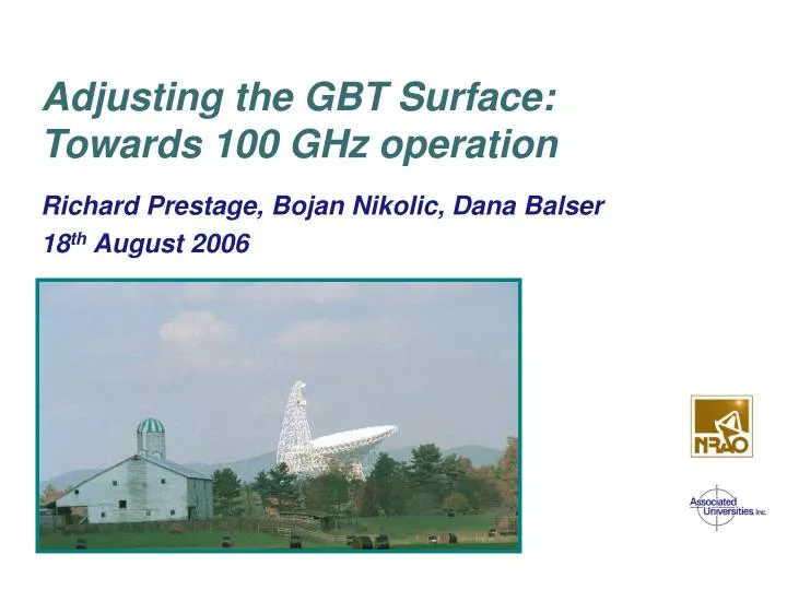
Adjusting the GBT Surface: Towards 100 GHz operation. Richard Prestage, Bojan Nikolic, Dana Balser 18 th August 2006. How to make a 100m telescope work at 50 GHz. … on the way to 115 GHz Pointing and surface accuracy are equally challenging

E N D
Adjusting the GBT Surface: Towards 100 GHz operation Richard Prestage, Bojan Nikolic, Dana Balser 18th August 2006
How to make a 100m telescope work at 50 GHz • … on the way to 115 GHz • Pointing and surface accuracy are equally challenging • I will only talk about surface accuracy today, pointing is a whole other story
Overview of talk • Review basic theory / causes of loss of telescope efficiency • Briefly describe basic “Phase I” GBT solutions • Describe the technique of phase retrieval (“out-of-focus”) holography and its application to the GBT
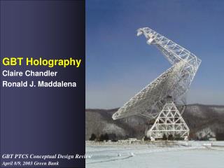
Acknowledgements • Everyone who has worked on the active surface (most recently Jason Ray, J.D. Nelson, Melinda Mello, Fred Schwab). • Richard Hills and colleagues who developed the analysis approach we use here • Bill Saxton for the line graphics for this talk
Performance Metrics Telescope performance can be quantified by two main quantities: • Image quality / efficiency: • PSF / Strehl ratio (optical) • Beam shape / aperture efficiency (radio) • Ability to point it in the right direction Image quality is determined by accuracy and alignment of the optics
Image quality and efficiency Theoretical beam pattern (point spread function) defined by Geometric Theory of Diffraction Aperture efficiency: η = Power collected by feed Power incident on antenna Max. value: η = 1
Quantifying telescope performance • Two theorems: • Reciprocity Theorem: Angular response of a radio telescope when used as a transmitting antenna is the same as when it is used as a receiving antenna • Fourier Transform theorem: Far field electric field pattern is the Fourier transform of the aperture plane distribution • Two main causes of loss: • Losses related to the amplitude of the electric field • Losses due to the phase of the electric field • See Goldsmith Single-Dish Summer School Lecture for excellent overview of these topics
Reciprocity Theorem Performance of the antenna when collecting radiation from a point source at infinity may be studied by considering its properties as a transmitter
Fourier transform relationship Far-field beam pattern is Fourier transform of aperture plane electric field distribution
Aperture plane Ideal telescope: ηa = 1 . 1 . 1 . 1 Real telescope: ηa = ηbηt ηs ηp 0.8 x 0.8 x 0.8 x 0.8 = 0.41 • Losses: • Blockage efficiency: ηb • Taper efficiency: ηt • Spillover efficiency: ηs • Phase efficiency: ηp
Blockage efficiency Effelsberg 100 m NRAO 140 Foot Conventional Telescope: ηb = 0.85 – 0.9 GBT: ηb = 1.0
Illumination efficiency – taper and spillover Idealized uniform illumination
Illumination efficiency – taper and spillover • blue = taper loss, red = spillover loss • Gaussian-illuminated zero phase error unblocked circular antenna: • ηa = ηt ηs=0.815 (maximum) for 11dB edge taper • ηa = ηt ηs = ~ 0.7 for ~15dB edge taper (GBT)
real telescope with phase losses Amplitude of electric field is largely unchanged Irregularities (deformations) in mirrors and misalignments cause phase errors => phase losses. Large scale errors (mis-alignments) may have predictable effects on beam pattern (e.g. astigmatism) Distribution of small-scale errors is generally unknown
real telescope with phase losses Error distribution modeled by Ruze Ruze formula: ε = rms surface error ηp = exp[(-4πε/λ)2] “pedestal” θp ~ Dθ/L ηa down by 3dB for ε = λ/16 “acceptable” performance ε = λ/4π
Summary • Maximum aperture efficiency ηt ηs (feed illumination) ~ 0.7 • Large-scale phase errors (e.g. misalignment of secondary) affect main beam and near-in side lobes • Random surface errors cause loss of efficiency and large scale error pedestal • Can use Ruze formula to define equivalent wavefront error
Scientific Requirements (GHz)
Challenges for large telescope design How do you achieve 200 µm accuracy – the thickness of two human hairs –over a 100m diameter surface –anarea equal to 21/4 football fields ?
What is possible? The Astronomical Journal, February 1967
Solutions… The Astronomical Journal, February 1967
GBT Solutions… • Innovative design/construction • Careful initial alignment • Active surface / FE model • Calibration measurements of residuals (OOF holography) • Real-time monitoring/dynamic adjustments (OOF holography) <= Original <= Now <= Future (Potential alternative: use laser rangefinders to measure absolute position of all optical elements and correct appropriately.)
Focus Tracking • Changing parabola causes change in location of prime focus (focal length changes, parabola “slides downhill”) • Feedarm also flexes under gravity • Six degree of freedom (Stewart platform) subreflector mount relocates subreflector to correct position
Subreflector focus tracking X,Y,Z = A + B cos(el) + C sin(el) Xt, Zt = Const
GBT active surface system • Surface has 2004 panels • average panel rms: 68 µm • 2209 precision actuators Operates in open loop from look-up table generated from Finite Element Model + OOF corrections
Surface Panel Actuators One of 2209 actuators. • Actuators are located under each set of surface panel corners • Actuator Control Room • 26,508 control and supply wires terminated in this room
Photogrammetry • Basis for setting actuator zero-points at “rigging angle” (~ 50 degrees) • Sets lower-limit on small-scale (panel to panel) error of around ~ 250 µm
FE Model - Efficiency and Beam Shape Focus tracking and FE Model: Acceptable surface to 20GHz
Phase II – “Out of focus” holography
Traditional (phase-reference) holography • Dedicated receiver to look at (usually) a terrestrial transmitter (at low elevation) or geostationary satellite • Second dish (or reference antenna) provides phase reference • Measure amplitude and phase of (near or far)-field beam pattern • Fourier transform to determine amplitude and phase of aperture illumination
Alternative – phase-retrieval holography • There are many advantages to traditional holography, but also some disadvantages: • Needs extra instrumentation • Reference antenna needs to be close by so that atmospheric phase fluctuations are not a problem • S/N ratio required limits sources to geostationary satellites, which are at limited elevation ranges for the GBT (35°-45°) • Alternative: measure power (instead of phase and amplitude) only, recover phase by modeling
“out-of-focus” holography • Hills, Richer, & Nikolic (Cavendish Astrophysics, Cambridge) have proposed a new technique for phase-retrieval holography. It differs from “traditional” phase-retrieval holography in three ways: • It describes the antenna surface in terms of Zernike polynomials and solves for their coefficients, thus reducing the number of free parameters • It uses modern minimization algorithms to fit for the coefficients • It recognizes that defocusing can be used to lower the S/N requirements for the beam maps
Some mathematics • Consider the combination of a perfect parabolic antenna with aperture function A0, and phase errors Q(k). • If Q small, A » A0(1+ iQ), and the far-field electric field pattern is E = FT [A0(1+ iQ)] = E0 + i[E0 ÄFT (Q)] = E0 + iF (defining F = E0 ÄFT (Q); F contains all the information about Q) • Power pattern of the antenna is then P = |E0|2 + |F|2 + 2[Á(E0)Â(F) - Â(E0)Á(F)] • Small defocus Þ last term is negligible, and Q is derived from fitting for |F|2 • Large defocus Þ end term dominates and different defocus values weight Â(F) and Á(F) differently to obtain independent information about F
Technique • Make three Nyquist-sampled beam maps, one in focus, one each ~ five wavelengths radial defocus • Model surface errors (phase errors) as combinations of low-order Zernike polynomials. Perform forward transform to predict observed beam maps (correctly accounting for phase effects of defocus) • Sample model map at locations of actual maps (no need for regridding) • Adjust coefficients to minimize difference between model and actual beam maps.
Technique • Typically work at Q-band (43 GHz in continuum) • Some tests done at Ka-band • Observe brightest calibrators in sky (e.g. 3C273), sources ~10 Jy • Data acquisition takes ~ 30 minutes • Data analysis takes ~ 10 minutes
Zernike polynomials z2: phase gradient (pointing shift) z5: astigmatism z8: coma aperture plane
Typical data Q-band (43 GHz)