Download
1 / 44
440 likes | 592 Views
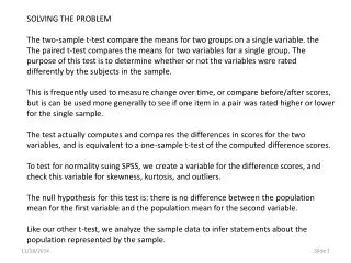
SOLVING THE PROBLEM The two-sample t-test compare the means for two groups on a single variable. the

E N D
SOLVING THE PROBLEM The two-sample t-test compare the means for two groups on a single variable. the The paired t-test compares the means for two variables for a single group. The purpose of this test is to determine whether or not the variables were rated differently by the subjects in the sample. This is frequently used to measure change over time, or compare before/after scores, but is can be used more generally to see if one item in a pair was rated higher or lower for the single sample. The test actually computes and compares the differences in scores for the two variables, and is equivalent to a one-sample t-test of the computed difference scores. To test for normality suing SPSS, we create a variable for the difference scores, and check this variable for skewness, kurtosis, and outliers. The null hypothesis for this test is: there is no difference between the population mean for the first variable and the population mean for the second variable. Like our other t-test, we analyze the sample data to infer statements about the population represented by the sample.
The introductory statement in the question indicates: • The data set to use (GSS2000R) • The variables to use in the analysis: confidence in the executive branch of the federal government [confed] and confidence in the United States Supreme Court [conjudge] • The task to accomplish (a paired t-test) • The level of significance (0.05, two-tailed)
The first statement asks about the level of measurement. A paired t-test requires that both variables be quantitative.
"Confidence in the executive branch of the federal government" [confed] is quantitative and "confidence in the United States Supreme Court" [conjudge] is quantitative, satisfying the level of measurement requirement. Mark the statement as correct.
To justify the use of probabilities based on a normal sampling distribution in testing hypotheses, either the distribution of the variable must satisfy the nearly normal condition or the size of the sample must be sufficiently large to generate a normal sampling distribution under the Central Limit Theorem. A paired t-test requires that the distribution of the paired differences between the variables satisfy the nearly normal condition, which we will operationally define as having skewness and kurtosis between -1.0 and +1.0, and having no outliers with standard scores equal to or smaller than -3.0 or equal to or larger than +3.0.
To evaluate the variables conformity to the nearly normal condition in a paired t-test, we must compute a difference variable by subtracting the second variable from the first variable. To start, select the Compute Variable command from the Transform menu.
We will name the new variable differences by typing the name in the Target Variable text box. In the Numeric Expression text box, we type the first variable minus the second variable.
To evaluate the variables conformity to the nearly normal condition, we compute descriptive statistics and standard scores for the difference variable. To compute the descriptive statistics and standard scores, select the Descriptive Statistics > Descriptives command from the Analyze menu.
Move the variable for the analysis differences to the Variable(s) list box. Click on the Options button to select optional statistics.
The check boxes for Mean and Std. Deviation are already marked by default. Click on Continue button to close the dialog box. Mark the Kurtosis and Skewness check boxes. This will provide the statistics for assessing normality.
Click on the OK button to produce the output. Mark the check box Save standardized values as variables.
"Paired differences between confidence in the executive branch of the federal government and confidence in the United States Supreme Court" satisfied the criteria for a normal distribution. The skewness of the distribution (-0.073) was between -1.0 and +1.0. The kurtosis of the distribution (0.563) was between -1.0 and +1.0.
Sort the column Zdifferencesin ascending order to show any negative outliers at the top of the column. There were no outliers that had a standard score less than or equal to -3.0.
Sort the column Zdifferencesin descending order to show any positive outliers at the top of the column. There were two outliers that had a standard score less than or equal to -3.0 or greater than or equal to +3.0: - 20000029 with a value of 2 (z=3.07) - 20001379 with a value of 2 (z=3.07)
Since it is unusual to have an outlier for the difference between two likert scale items, I looked at the combination of scores that would produce an outlier. These two cases had a great deal (3) of confidence in the executive branch and hardly any (1) confidence in the supreme court.
Because of the presence of outliers, we do not satisfy the nearly normal condition for the difference variable. The check box is not marked.
Since we cannot justify the use of probabilities based on a normal sampling distribution by satisfying the nearly normal condition, we will try applying the Central Limit Theorem. To apply the Central Limit Theorem for a paired t-test requires that the sample contain 40 or more cases.
The number of valid cases available for the test was 172, larger than requirement of 40 cases to apply the Central Limit Theorem. Since the distribution did not satisfy the nearly normal condition, we will rely upon the Central Limit Theorem to satisfy the sampling distribution requirements of a paired t-test.
Since the number of valid cases available for the test was larger than requirement of 40 cases to apply the Central Limit Theorem, we mark the statement as correct.
The next statement asks us to identify the mean difference and the standard error of the sampling distribution of differences. To answer this question, we need to produce the output for the paired t-test.
To produce the paired t-test, select the Compare Means > Paired-Samples T Test command from the Analyze menu.
For the paired t-test, we have to select the two variables for the test and move them as a pair. Click on the first variable name, confed, and it moves to the Current Selections panel. If you move the wrong variable, click on its name a second time to de-select it, or you can click on the Reset button.
With the pair of variables selected, click on the right arrow button to move the variables to the Paired Variables list box. Click on the second variable name, conjudge, and it moves to the Current Selections panel.
The correct value for the mean was -0.314. The standard error of the paired differences was 0.057.
The correct value for the mean was -0.314. The standard error of the paired differences was 0.057. Mark the check box as correct.
The next statement asks us about the null hypothesis for the paired t-test. We should check to make certain the relationship is stated correctly for the test.
The null hypothesis for a paired t-test states that there is no difference between the population mean for "confidence in the executive branch of the federal government" and the population mean for "confidence in the United States Supreme Court". The hypothesis states that the average difference is equal to 0 for paired scores for "confidence in the executive branch of the federal government" and "confidence in the United States Supreme Court". Mark the statement as correct.
The next statement asks us to relate the t-test to the data in our problem.
The t-test statistic is based on the mean difference between paired scores on the two variables (-0.314) relative to the standard error of the paired differences between sample means (0.057). Both values are identified correctly.
The t-test statistic is based on the mean difference between paired scores on the two variables (-0.314) relative to the standard error of the paired differences between sample means (0.057). Mark the statement as correct.
The next statement asks about the probability for the comparison made by the t-test. i.e. what is the probability that the differences in the ratings for the two variables was equal to zero.
The probability that the mean difference between paired scores in the population was equal to 0 was p < .001.
The probability was p < .001 that the mean difference between paired scores in the population was equal to 0. Mark the statement as correct.
When the p-value for the statistical test is less than or equal to alpha, we reject the null hypothesis and interpret the results of the test. If the p-value is greater than alpha, we fail to reject the null hypothesis and do not interpret the result.
The p-value for this test (p < .001) is less than or equal to the alpha level of significance (p = .050) supporting the conclusion to reject the null hypothesis. Mark the check box as correct.
The final statement asks us to interpret the result of our statistical test as a finding in the context of the problem we created. We only interpret the results when the null hypothesis is rejected.
The mean for "confidence in the executive branch of the federal government" [confed] (1.808) is actually smaller than the mean for "confidence in the United States Supreme Court" [conjudge] (2.122).
Since we rejected the null hypothesis and since the mean for "confidence in the executive branch of the federal government" [confed] (1.808) is actually smaller than the mean for "confidence in the United States Supreme Court" [conjudge] (2.122), it is reasonable to suggest that survey respondents had less confidence in the executive branch of the federal government than they had in the U. S. Supreme Court. Mark the check box as correct.
Variables are quantitative? Do not mark check box. No Mark only “None of the above.” Stop. Mark statement check box. Compute difference variable. Yes
Difference variable nearly normal distribution? • Nearly normal: • Skewness between -1.0 and +1.0 • Kurtosis between -1.0 and +1.0 • Z-scores between -3.0 and +3.0 Do not mark check box. No CLT stands for Central Limit Theorem. CLT applicable (Sample size ≥ 40)? Mark statement check box. Do not mark check box. CLT applicable (Sample size ≥ 40)? Stop. Yes No Yes Yes No If the difference variable is not normal and the sample size is less than 40, the test is not appropriate. Do not mark check box. Mark statement check box. The path is complicated because we check two conditions, but only one needs to be correct to continue.
Mean difference and standard error correct? Do not mark check box. No Mark statement check box. H0: mean difference = 0 Do not mark check box. No Yes Yes Mark statement check box.
T-test accurately described? Do not mark check box. No Mark statement check box. P-value (sig.) stated correctly? Do not mark check box. No Yes Yes Mark statement check box.
Reject H0 is correct decision (p ≤ alpha)? Do not mark check box. No Stop. We interpret results only if we reject null hypothesis. Mark statement check box. Interpretation is stated correctly? Do not mark check box. No Yes Yes Mark statement check box.