Download
1 / 12
140 likes | 288 Views
Simulation Model for Mobile Radio Channels. Ciprian Romeo Com şa Iolanda Alecsandrescu Andrei Maiorescu Ion Bogdan ccomsa@etc.tuiasi.ro. Technical University “Gh. Asachi” Ia ş i Department of Telecommunications. Radio channel.

E N D
Simulation Model for Mobile Radio Channels Ciprian Romeo Comşa Iolanda Alecsandrescu Andrei Maiorescu Ion Bogdan ccomsa@etc.tuiasi.ro Technical University “Gh. Asachi” Iaşi Department of Telecommunications
Radio channel Radio channel: propagation medium characterized by wave phenomena. Diffraction Reflection Scattering
Fading The propagation is realized mostly by reflection and diffraction. Waves are received on different propagation ways => Multi-path Propagation. The sum of waves received may have significant variations even on slow motion of receiver. This is called short-term fading or fast fading and follows a Rayleigh distribution. Diffraction LOS propagation Reflection
Fading The propagation is realized mostly by reflection and diffraction. Waves are received on different propagation ways => Multi-path Propagation. The sum of waves received may have significant variations even on slow motion of receiver. This is called short-term fading or fast fading and follows a Rayleigh distribution. The mean of the received signal has slow variations on larger motion. This is called long-term fading and follows a log-normal distribution. Short-term fading Long-term fading
Channel Modeling • A channel model has to allow the evaluation of the propagation loses and theirs variations (fading). • The Suzuki model takes into account short-term fading with superimposed long-term log-normal variations of the mean of received signal:
Analytical model – Stochastic process: • models the short-time fading • is obtained considering: • complex zero mean Gaussian noise process with cross-correlated quadrature components and • LOS component supposed to be independent of time (for short-time fading) • is obtained as envelope of nonzero mean Gaussian noise process • For particular values of environment parameters, this process follows Rice, Rayleigh or one-sided Gaussian distribution. Extended Suzuki Stochastic process Log-normal process
Analytical model – Log-normal process: • models the long-time fading, caused by shadowing effects • is obtained from another real Gaussian noise process with zero mean and unit variance: • m and s are two environment parameters • and are uncorrelated Extended Suzuki Stochastic process Log-normal process
Simulation Model • cross-correlated • Simulation coefficients: • -Doppler coefficients • -discrete Doppler frequencies • - Doppler phases • = number of sinusoids used to approximate the Gaussian processes
Simulation • A mixed signal simulation tool is used – Saber Designer with MAST language • MAST = HDL => the channel model can be used for simulations deeper to hardware systems Simulation Data • Environment parameters: • Number of sinusoids: N1=25 and N2=15. • Number of samples NS=108 and sampling period Ta=3·10-8s. • Maximum Doppler frequency fmax=91Hz, corresponding to a vehicle’s speed of 110Km/h. • Doppler coefficients ci,n and discrete Doppler frequencies fi,n are calculated at the beginning and kept constants during the simulation. • Doppler phases θi,n are modified at each simulation step given by sampling.
Simulation results (1) Envelope of the simulated extended Suzuki process
Simulation results (2) • The differences between the generated signal distribution obtained as histogram and the analytical pdf are hardly observable. • The values for mean and standard deviation confirms this affirmation.
Conclusion Histogram of simulated extended Suzuki model, in cases of: • Light shadowing log-normal distribution • Heavy shadowing Rice (or Rayleigh) distribution