BINARY CHOICE MODELS: PROBIT ANALYSIS

1. BINARY CHOICE MODELS: PROBIT ANALYSIS In the case of probit analysis, the sigmoid function is the cumulative standardized normal distribution. 1

2. BINARY CHOICE MODELS: PROBIT ANALYSIS The maximum likelihood principle is again used to obtain estimates of the parameters. 2

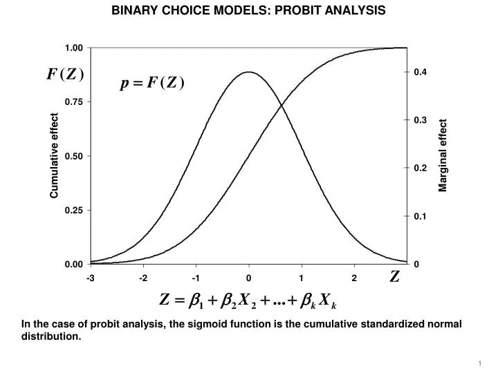
3. BINARY CHOICE MODELS: PROBIT ANALYSIS . probit GRAD ASVABC SM SF MALE Iteration 0: log likelihood = -118.67769 Iteration 1: log likelihood = -98.195303 Iteration 2: log likelihood = -96.666096 Iteration 3: log likelihood = -96.624979 Iteration 4: log likelihood = -96.624926 Probit estimates Number of obs = 540 LR chi2(4) = 44.11 Prob > chi2 = 0.0000 Log likelihood = -96.624926 Pseudo R2 = 0.1858 ------------------------------------------------------------------------------ GRAD | Coef. Std. Err. z P>|z| [95% Conf. Interval] -------------+---------------------------------------------------------------- ASVABC | .0648442 .0120378 5.39 0.000 .0412505 .0884379 SM | -.0081163 .0440399 -0.18 0.854 -.094433 .0782004 SF | .0056041 .0359557 0.16 0.876 -.0648677 .0760759 MALE | .0630588 .1988279 0.32 0.751 -.3266368 .4527544 _cons | -1.450787 .5470608 -2.65 0.008 -2.523006 -.3785673 ------------------------------------------------------------------------------ Here is the result of the probit regression using the example of graduating from high school. 3

4. BINARY CHOICE MODELS: PROBIT ANALYSIS . probit GRAD ASVABC SM SF MALE Iteration 0: log likelihood = -118.67769 Iteration 1: log likelihood = -98.195303 Iteration 2: log likelihood = -96.666096 Iteration 3: log likelihood = -96.624979 Iteration 4: log likelihood = -96.624926 Probit estimates Number of obs = 540 LR chi2(4) = 44.11 Prob > chi2 = 0.0000 Log likelihood = -96.624926 Pseudo R2 = 0.1858 ------------------------------------------------------------------------------ GRAD | Coef. Std. Err. z P>|z| [95% Conf. Interval] -------------+---------------------------------------------------------------- ASVABC | .0648442 .0120378 5.39 0.000 .0412505 .0884379 SM | -.0081163 .0440399 -0.18 0.854 -.094433 .0782004 SF | .0056041 .0359557 0.16 0.876 -.0648677 .0760759 MALE | .0630588 .1988279 0.32 0.751 -.3266368 .4527544 _cons | -1.450787 .5470608 -2.65 0.008 -2.523006 -.3785673 ------------------------------------------------------------------------------ As with logit analysis, the coefficients have no direct interpretation. However, we can use them to quantify the marginal effects of the explanatory variables on the probability of graduating from high school. 4

5. BINARY CHOICE MODELS: PROBIT ANALYSIS As with logit analysis, the marginal effect of Xi on p can be written as the product of the marginal effect of Z on p and the marginal effect of Xi on Z. 5

6. BINARY CHOICE MODELS: PROBIT ANALYSIS The marginal effect of Z on p is given by the standardized normal distribution. The marginal effect of Xi on Z is given by bi. 6

7. BINARY CHOICE MODELS: PROBIT ANALYSIS As with logit analysis, the marginal effects vary with Z. A common procedure is to evaluate them for the value of Z given by the sample means of the explanatory variables. 7

8. BINARY CHOICE MODELS: PROBIT ANALYSIS . sum GRAD ASVABC SM SF MALE Variable | Obs Mean Std. Dev. Min Max -------------+-------------------------------------------------------- GRAD | 540 .9425926 .2328351 0 1 ASVABC | 540 51.36271 9.567646 25.45931 66.07963 SM | 540 11.57963 2.816456 0 20 SF | 540 11.83704 3.53715 0 20 MALE | 540 .5 .5004636 0 1 As with logit analysis, the marginal effects vary with Z. A common procedure is to evaluate them for the value of Z given by the sample means of the explanatory variables. 8

9. BINARY CHOICE MODELS: PROBIT ANALYSIS Probit: Marginal Effects mean b product f(Z) f(Z)b ASVABC 51.36 0.065 3.328 0.068 0.004 SM 11.58 –0.008 –0.094 0.068 –0.001 SF 11.84 0.006 0.066 0.068 0.000 MALE 0.50 0.063 0.032 0.068 0.004 constant 1.00 –1.451–1.451 Total 1.881 In this case Z is equal to 1.881 when the X variables are equal to their sample means. 9

10. BINARY CHOICE MODELS: PROBIT ANALYSIS Probit: Marginal Effects mean b product f(Z) f(Z)b ASVABC 51.36 0.065 3.328 0.068 0.004 SM 11.58 –0.008 –0.094 0.068 –0.001 SF 11.84 0.006 0.066 0.068 0.000 MALE 0.50 0.063 0.032 0.068 0.004 constant 1.00 –1.451–1.451 Total 1.881 We then calculate f(Z). 10

11. BINARY CHOICE MODELS: PROBIT ANALYSIS Probit: Marginal Effects mean b product f(Z) f(Z)b ASVABC 51.36 0.065 3.328 0.068 0.004 SM 11.58 –0.008 –0.094 0.068 –0.001 SF 11.84 0.006 0.066 0.068 0.000 MALE 0.50 0.063 0.032 0.068 0.004 constant 1.00 –1.451–1.451 Total 1.881 The estimated marginal effects are f(Z) multiplied by the respective coefficients. We see that a one-point increase in ASVABC increases the probability of graduating from high school by 0.4 percent. 11

12. BINARY CHOICE MODELS: PROBIT ANALYSIS Probit: Marginal Effects mean b product f(Z) f(Z)b ASVABC 51.36 0.065 3.328 0.068 0.004 SM 11.58 –0.008 –0.094 0.068 –0.001 SF 11.84 0.006 0.066 0.068 0.000 MALE 0.50 0.063 0.032 0.068 0.004 constant 1.00 –1.451–1.451 Total 1.881 Every extra year of schooling of the mother decreases the probability of graduating by 0.1 percent. Father's schooling has no discernible effect. Males have 0.4 percent higher probability than females. 12

13. BINARY CHOICE MODELS: PROBIT ANALYSIS Logit Probit Linear f(Z)b f(Z)b b ASVABC 0.004 0.004 0.007 SM–0.001 –0.001 –0.002 SF 0.000 0.000 0.001 MALE 0.004 0.004 –0.007 The logit and probit results are displayed for comparison. The coefficients in the regressions are very different because different mathematical functions are being fitted. 13

14. BINARY CHOICE MODELS: PROBIT ANALYSIS Logit Probit Linear f(Z)b f(Z)b b ASVABC 0.004 0.004 0.007 SM–0.001 –0.001 –0.002 SF 0.000 0.000 0.001 MALE 0.004 0.004 –0.007 Nevertheless the estimates of the marginal effects are usually similar. 14

15. BINARY CHOICE MODELS: PROBIT ANALYSIS Logit Probit Linear f(Z)b f(Z)b b ASVABC 0.004 0.004 0.007 SM–0.001 –0.001 –0.002 SF 0.000 0.000 0.001 MALE 0.004 0.004 –0.007 However, if the outcomes in the sample are divided between a large majority and a small minority, they can differ. 15

16. BINARY CHOICE MODELS: PROBIT ANALYSIS Logit Probit Linear f(Z)b f(Z)b b ASVABC 0.004 0.004 0.007 SM–0.001 –0.001 –0.002 SF 0.000 0.000 0.001 MALE 0.004 0.004 –0.007 This is because the observations are then concentrated in a tail of the distribution. Although the logit and probit functions share the same sigmoid outline, their tails are somewhat different. 16

17. BINARY CHOICE MODELS: PROBIT ANALYSIS Logit Probit Linear f(Z)b f(Z)b b ASVABC 0.004 0.004 0.007 SM–0.001 –0.001 –0.002 SF 0.000 0.000 0.001 MALE 0.004 0.004 –0.007 This is the case here, but even so the estimates are identical to three decimal places. According to a leading authority, Amemiya, there are no compelling grounds for preferring logit to probit or vice versa. 17

18. BINARY CHOICE MODELS: PROBIT ANALYSIS Logit Probit Linear f(Z)b f(Z)b b ASVABC 0.004 0.004 0.007 SM–0.001 –0.001 –0.002 SF 0.000 0.000 0.001 MALE 0.004 0.004 –0.007 Finally, for comparison, the estimates for the corresponding regression using the linear probability model are displayed. 18

19. BINARY CHOICE MODELS: PROBIT ANALYSIS Logit Probit Linear f(Z)b f(Z)b b ASVABC 0.004 0.004 0.007 SM–0.001 –0.001 –0.002 SF 0.000 0.000 0.001 MALE 0.004 0.004 –0.007 If the outcomes are evenly divided, the LPM coefficients are usually similar to those for logit and probit. However, when one outcome dominates, as in this case, they are not very good approximations. 19

20. Binary Response Models: Interpretation II • Probit: g(0)=.4 • Logit: g(0)=.25 • Linear probability model: g(0)=1 • To make the logit and probit slope estimates comparable, we can multiply the probit estimates by .4/.25=1.6. • The logit slope estimates should be divided by 4 to make them roughly comparable to the LPM (Linear Probability Model) estimates.