Download

1 / 27
330 likes | 635 Views
Linear Classifier. Team teaching. Linear Methods for Classification. Lecture Notes for CMPUT 466/551 Nilanjan Ray. Linear Classification. What is meant by linear classification? The decision boundaries in the in the feature (input) space is linear Should the regions be contiguous?. R 1.

E N D
Linear Classifier Team teaching
Linear Methods for Classification Lecture Notes for CMPUT 466/551 Nilanjan Ray
Linear Classification • What is meant by linear classification? • The decision boundaries in the in the feature (input) space is linear • Should the regions be contiguous? R1 R2 X2 R3 R4 X1 Piecewise linear decision boundaries in 2D input space
Linear Classification… • There is a discriminant functionk(x) for each class k • Classification rule: • In higher dimensional space the decision boundaries are piecewise hyperplanar • Remember that 0-1 loss function led to the classification rule: • So, can serve as k(x)
Linear Classification… • All we require here is the class boundaries {x:k(x) = j(x)} be linear for every (k, j) pair • One can achieve this if k(x) themselves are linear or any monotone transform of k(x) is linear • An example: So that Linear
Linear Discriminant Analysis Essentially minimum error Bayes’ classifier Assumes that the conditional class densities are (multivariate) Gaussian Assumes equal covariance for every class Posterior probability Application of Bayes rule kis the prior probability for class k fk(x) is class conditional density or likelihood density
LDA… Classification rule: is equivalent to: The good old Bayes classifier!
LDA… When are we going to use the training data? Total N input-output pairs Nk number of pairs in class k Total number of classes: K Training data utilized to estimate Prior probabilities: Means: Covariance matrix:
LDA: Example LDA was able to avoid masking here
Study case • Factory “ABC” produces very expensive and high quality chip rings that their qualities are measured in term of curvature and diameter. Result of quality control by experts is given in the table below.
As a consultant to the factory, you get a task to set up the criteria for automatic quality control. Then, the manager of the factory also wants to test your criteria upon new type of chip rings that even the human experts are argued to each other. The new chip rings have curvature 2.81 and diameter 5.46. • Can you solve this problem by employing Discriminant Analysis?
Solutions • When we plot the features, we can see that the data is linearly separable. We can draw a line to separate the two groups. The problem is to find the line and to rotate the features in such a way to maximize the distance between groups and to minimize distance within group.
X = features (or independent variables) of all data. Each row (denoted by ) represents one object; each column stands for one feature. • Y = group of the object (or dependent variable) of all data. Each row represents one object and it has only one column.
Xk = data of row k, for example x3 = • g=number of gropus in y, in our example, g=2 • Xi = features data for group i . Each row represents one object; each column stands for one feature. We separate x into several groups based on the number of category in y.
μi = mean of features in group i, which is average of xi • μ1 = , μ2 = • μ = global mean vector, that is mean of the whole data set. • In this example, μ =
= mean corrected data, that is the features data for group i, xi , minus the global mean vector μ = =
Covariance matrix of group i = C1 = C2 =
= pooled within group covariance matrix. It is calculated for each entry in the matrix. In our example, 4/7*0.166 + 3/7*0.259=0.206 , 4/7*(-0.192)+3/7*(-0.286)=-0.233 and 4/7*1.349+3/7*2.142=1.689 , therefore
C = The inverse of covariance matrix is : C-1 =
P = prior probability vector (each row represent prior probability of group ). If we do not know the prior probability, we just assume it is equal to total sample of each group divided by the total samples, that is p = =
discriminant function • We should assign object k to group i that has maximum fi
Tugas • Gunakan excel/matlab/tools lain untuk mengklasifikasi data set breast tissue secara : • Naïve Bayes • LDA Presentasikan minggu depan