Download
1 / 66
660 likes | 792 Views
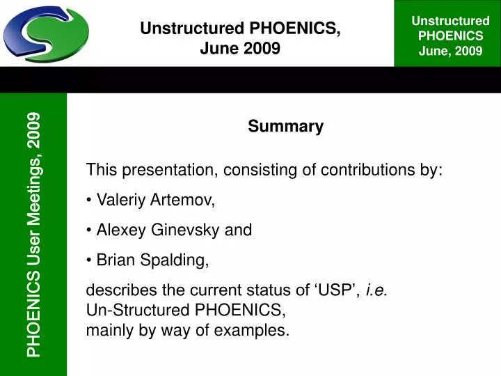
Unstructured PHOENICS, June 2009. Summary. This presentation, consisting of contributions by: Valeriy Artemov, Alexey Ginevsky and Brian Spalding, describes the current status of ‘USP’, i.e. Un-Structured PHOENICS, mainly by way of examples. Contents list.

E N D
Unstructured PHOENICS,June 2009 Summary • This presentation, consisting of contributions by: • Valeriy Artemov, • Alexey Ginevsky and • Brian Spalding, • describes the current status of ‘USP’, i.e. • Un-Structured PHOENICS, • mainly by way of examples.
Contents list The topics considered include: • why USP is being developed (slide 3) • general description (slide 5) • how the grids are generated (slide 6) • examples of unstructured-grid flow simulations (slides 9, 14, 17 and 22) • comparisons with structured PHOENICS ( i.e. SP) (slide 31) • applications to terrain-type flow simulations (slide 35) • applications to solid-stress simulations (slide 56) • the (not-yet-incorporated) smoothing algorithm for boundary cells • (slide 59).
Why USP is being developed:economy of computer time & storage The motive for introducing it has not been (as it may be for competitors) to handle curved-surface bodies; for PARSOL handles these satisfactorily. Instead, the motive is to reduce the waste of time and storage entailed by the un-needed fine-grid regions which PHOENICS (in structured- grid mode) generates far from the bodies, as seen on the right. For the hollow-box heat-conduction problem on the left, SP (structured PHOENICS) pays attention also to the empty central volume; USP does not.
Another example of USP’s ignoring unimportant regions Here is shown a non-straight duct contained within a solid block. To compute the flow within it, SP uses a grid which covers the whole block. Moreover it repeatedly visits all cells in the grid and re-computes the (zero) velocities in the solid. USP, by contrast, has few cells in the solid region, or even none at all; and it makes calculations only for cells which lie within the duct. (See library case u009)
General description;the unstructured grid USP is a part of the standard PHOENICS package, which can therefore work in structured or unstructured modes at user’s choice. Setting USP=T in the Q1 file is the first step. Then the user must make decisions about the computational grid which is to be used. All USP grids consist of Cartesian (i.e.) brick-shaped cells. The general polygonal shapes such as this used in other codes have been judged to be needlessly complex. USP cells adjoining objects with curved surfaces can be distorted so as to fit them better, as shown on the right rectangular distorted
General description;how the grid is created USP employs a standard-PHOENICS cartesian grid as its starting point. If this is a very fine one it proceeds by coarsening, i.e. by replacing pairs, quartets or octets of cells by single cells, until the required economical grid is arrived at. Alternatively, it may start from an already coarse grid and proceed by refining it, i.e. by halving cells systematically until the grid is sufficiently fine in the regions of special interest. The recently-developed AGG (Automatic Grid Generator) module proceeds by way refinement, guided by settings made by the user and by what VR-objects it finds to have been introduced. AGG is described in more detail elsewhere (AGG.ppt)
General description;the unstructured grid Unstructured grids may look, in two dimensions like this This is the grid which is used for the two-sphere comparison below. In a USP grid, faces of larger cells may adjoin 2 smaller cells, or 4 in three-dimensional cases, but no more.
General description;another 2D grid This grid was created by means of AGG, the Automatic Grid Generator, a utility program which is supplied with the PHOENICS package. AGG detects the presence, size and location of facetted ‘virtual-reality’ objects, and then fits layers of small cells to their surfaces.
Examples of unstructured-grid flow simulationswith AGG-generated grids • The examples concern: • heat conduction, two-dimensional • heat conduction, three-dimensional • flow around a cylinder • Mixing hot and cold water in a faucet (tap)
USP and AGG: Example #12D Heat conduction in plate with holes A plate is perforated by holes and slots. Heat is conducted from the top boundary at 10 degrees to the bottom boundary at 0 degrees. The coarse grid from which AGG starts is shown by the dark lines.
USP and AGG: Example #12D Heat conduction AGG, following a few user-given instructions in the Q1 file concerning number of refinement levels and how manylayers of cells are to be used at each level, then creates the grid shown on the right. Cells are smallest at hole and slot surfaces.
USP and AGG: Example #1;the results of calculation The resulting temperature contours reveal the expected effects: the slots and holes serve as barriers to the flow of heat. Of course, structured PHOENICS could have solved this problem easily with a uniformly fine grid, but at greater expense.
USP and AGG: Example #1In-Form ‘stored’ statement Most In-Form statements work for USP in the same way as for SP. Here are shown contours of A001, defined by: (STORED of A001 is Rho1*SQRT(XG^2+YG^2) with SWPFIN)
USP and AGG: Example #2;3D Heat conduction • Heat flows from the bottom boundary of a hollow 3D object • at 10 degrees C • to the top boundary • at 0 degrees C. • If SP were used: • a fine grid would have to be used for the whole of the bounding-box space • most of the computing time would have beenwasted.
USP and AGG: Example #2“Heat conduction” On the right are shown the cells which touch the inner and outer surfaces of the solid body. They are of a uniformly small size. Larger cells fill the remainder of the volume of the object. No cells exist at all in the non-solid spaces. AGG has therefore built a grid of maximum economy. Cell distortion for better fitting is not used here.
USP and AGG: Example #2Computed temperature distribution The temperature contours are shown on the right. Part of the body has been cut away in order that the contours on the inner surface can be seen. If there had been fluid inside and outside the body, AGG would have created cells in those regions also. Then USP would have calculated the temperatures there too; and also velocities and pressures, there only.
USP and AGG: Example #3;Flow around a cylinder Flow is present in this third example which concerns steady laminar flow around a cylinder within a duct of finite width, from left to right. The geometry is 2D. The Reynolds number is 40. AGG starts with the coarse grid.
USP and AGG: Example #3;the unstructured grid AGG created this grid, with smallest cells nearest to the surface
USP and AGG: Example #3Computed velocity vectors The closeness of the vectors reveals the local grid fineness
USP and AGG: Example #4;faucet for mixing hot and cold water Structured PHOENICS could have handled example #3 quite well; but it would be extremely inefficient if applied to example #4 . The object represents a domestic hot-&-cold-water tap. Only internal passages require CFD analysis; but the solid partsconduct heat.
USP and AGG: Example #4Test case: T-channel • A preliminary calculation with simpler geometry was made first with both SP and USP, and with • mass fluxes and temperatures of water, and • size of channels also the same as in the Faucet.
USP and AGG: Example #4Test case: comparison of SP and USP Velocity vectors and temperature contours USP SP Note that SP and USP use different display software
USP and AGG: Example #4Test case: comparison of SP and USP Pressure contours P max = 22.2 P min = - 8.0 USP SP P max = 21.5 P min = - 7.0 So there are small differences.
USP and AGG: Example #4Grid and PRPS (material index) contours MaxLevel = 4; i.e. there are 4 levels of grid refinement. The total number of cells is: 174 000 The fluid space is coloured blue; the solid space is coloured olive.
USP and AGG: Example #4Temperature contours • The public-domain package PARAVIEW is here used for displaying temperature contours on: • two cutting planes, and • part of the outside of the faucet. • The temperature range is from 0 to 100 degrees.
USP and AGG: Example #4;surface-temperature contours A fictitious cylindrical object has been attached to the outlet so as to enable the outlet pressure to be specified
USP and AGG: Example #4;Velocity vectors (coloured by pressure) The arrows show the hot and cold entering streams, which flow towards each other. They then join and flow out together along the curved tube to the outlet.
Comparisons between SP and USP; fine-grid embedding Since the SP technique of fine-grid embeddingalready allows grids to have varied coarseness from place to place, comparison is possible and interesting. However, USP uses a collocated (i.e. not staggered) scheme for the pressure~velocity interactions; therefore some differences are to be expected. The flow around two spheres has been calculated in both structured and unstructured modes (Input-file-library case u208). For equal numbers of cells, the ratio of computer times was 333 : 72 . So USP was more than four times faster than SP. The results will now be displayed graphically.
Comparison USP via SP + FGEfor flow around two spheres; grids The SP grid, with fine-grid embedding is shown below The corresponding unstructured grid was as shown here (with a smaller scale)
Comparison USP via SP + FGEfor flow around two spheres: SP SP+FGE: results Elapsed time is 333 seconds on PC pentium-IV, 2.4 GHz
Comparison USP via SP + FGEfor flow around two spheres: SP USP: results Elapsed time is 72 seconds on PC pentium-IV, 2.4 GHz The results of SP and USP were essentially similar; but the latter were obtained much more rapidly.
Further comparisons of SP and USP;flow over terrain USP is particularly useful for flow-over-terrain problems,where fine grids are required near the ground, whereas coarser ones suffice for higher altitudes. For given fineness near the ground, USP uses fewer cells than SP. For the same number of cells, USP’s grid is finer near the ground. The results of two test cases are shown below: 1. Flow over a pyramid-shaped mountain 2. Flow over natural terrain.
Comparison of Structured and Unstructured PHOENICS Case 1. Flow around pyramid Size of domain: 10x10x4m Inlet Velocity: 1 m/s Effective viscosity: m**2/s Sizes of smallest cells are same for SP and USP Structured grid is uniform with 80x80x32= 204,800 cells. Unstructured grid has 29,778 cells 96,934 faces Refinement level = 4.
Case 1 Unstructured grid Z = 1 m Y = 4 m
Case 1 Convergence of USP LSWEEP = 150, Elapsed time = 51 seconds
Case 1 Convergence of SP LSWEEP = 150, Elapsed time = 458 seconds; So USP runs 8,98 times faster than SP
Case 1 Comparison of outcomes. Pressure at Z = 0. SP USP The maximum pressures are the same
Case 1 Comparison of outcomes. Velocity U1 at Z = 1 m SP USP Maxima and minima are the same
Case 1 Comparison of outcomes. Velocity U1 at Y = 4 m SP USP
Comparison of Structured and Unstructured PHOENICS Case 2. Flow above natural terrain Size of domain 9.0x7.5x1.2 km Inlet Velocity 1 m/s Effective viscosity 10 sq.m/sec Structured grid is uniform with 144x120x24, i.e. 414,720 cells. Unstructured grid has 77,382 cells i.e.19% of structured. 252,289 faces. Refinement level = 3 Sizes of smallest cells are the same for SP and USP.
Case 2 Unstructured grid at Z = 0 m at Z = 200 m Note that there are no cells beneath the ground surface
Case 2 Unstructured grid at Z = 400 m at Y = 3800 m The cells become larger with increased distance from the ground.
Case 2 Convergence of USP LSWEEP = 266, Elapsed time = 295 seconds
Case 2 Convergence of SP LSWEEP = 210, Elapsed time = 1792 seconds USP faster by 6.07 times even with more SWEEPs.
Case 2 Comparison of outcomes. Pressure at Z = 100 m. SP USP