ADT for Map:

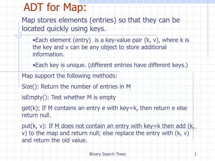
1. Map stores elements (entries) so that they can be located quickly using keys. • Each element (entry) is a key-value pair (k, v), where k is the key and v can be any object to store additional information. • Each key is unique. (different entries have different keys.) • Map support the following methods: • Size(): Return the number of entries in M • isEmpty(): Test whether M is empty • get(k); If M contains an entry e with key=k, then return e else return null. • put(k, v): If M does not contain an entry with key=k then add (k, v) to the map and return null; else replace the entry with (k, v) and return the old value. ADT for Map: Binary Search Trees

2. remove(k): remove from M the netry with key=k and return its value; if M has no such entry with key=k then return null. keys(); Return an iterable collection containing all keys stored in M values(): Return an iterable collection containing all values in M entries(): return an iterable collection containing all key-value entries in M. Remakrs: hash table is an implementation of Map. Methods of Map (continued) Binary Search Trees

3. A Dictionary stores elements (entries). • Each element (entry) is a key-value pair (k, v), where k is the key and v can be any object to store additional information. • The key is NOT unique. • Dictionary support the following methods: • size(): Return the number of entries in D • isEmpty(): Test whether D is empty • find(k): If D contains an entry e with key=k, then return e else return null. • findAll(k): Return an iterable collection containing all entries with key=k. • insert(k, v): Insert an entry into D, returning the entry created. • remove(e): remove from D an enty e, returing the removed entry or null if e was not in D. • entries(): return an iterable collection of the key-value entries in D. ADT for Dictionary: Binary Search Trees

4. Part-F1Binary Search Trees 6 < 2 9 > = 8 1 4 Binary Search Trees

5. Tree data structure that can be used to implement a dictionary. find(k): If D contains an entry e with key=k, then return e else return null. findAll(k): Return an iterable collection containing all entries with key=k. insert(k, v): Insert an entry into D, returning the entry created. remove(e): remove from D an enty e, returing the removed entry or null if e was not in D. Search Trees Binary Search Trees

6. A binary search tree is a binary tree storing keys (or key-value entries) at its internal nodes and satisfying the following property: Let u, v, and w be three nodes such that u is in the left subtree of v and w is in the right subtree of v. We have key(u)key(v) key(w) Different nodes can have the same key. External nodes do not store items An inorder traversal of a binary search trees visits the keys in increasing order 6 2 9 1 4 8 Binary Search Trees Binary Search Trees

7. Search AlgorithmTreeSearch(k, v) ifT.isExternal (v) returnv if k<key(v) returnTreeSearch(k, T.left(v)) else if k=key(v) returnv else{ k>key(v) } returnTreeSearch(k, T.right(v)) • To search for a key k, we trace a downward path starting at the root • The next node visited depends on the outcome of the comparison of k with the key of the current node • If we reach a leaf, the key is not found and we return null • Example: find(4): • Call TreeSearch(4,root) 6 < 2 9 > = 8 1 4 Binary Search Trees

8. Insertion 6 < • To perform operation insert(k, o), we search for key k (using TreeSearch) Algorithm TreeINsert(k, x, v): Input: A search key, an associate value x and a node v of T to start with Output: a new node w in the subtree T(v) that stores the entry (k, x) W TreeSearch(k,v) If k=key(w) then return TreeInsert(k, x, T.left(w)) T.insertAtExternal(w, (k, x)) Return • Example: insert 5 • Example: insert another 5? 2 9 > 1 4 8 > w 6 2 9 1 4 8 w 5 Binary Search Trees

9. Deletion 6 < • To perform operation remove(k), we search for key k • Assume key k is in the tree, and let v be the node storing k • If node v has a leaf child w, we remove v and w from the tree with operation removeExternal(w), which removes w and its parent and replace v with the remaining child. • Example: remove 4 2 9 > v 1 4 8 w 5 6 2 9 1 5 8 Binary Search Trees

10. Deletion (cont.) 1 v • We consider the case where the key k to be removed is stored at a node v whose children are both internal • we find the internal node w that follows v in an inorder traversal • we copy key(w) into node v • we remove node w and its left child z (which must be a leaf) by means of operation removeExternal(z) • Example: remove 3 3 2 8 6 9 w 5 z 1 v 5 2 8 6 9 Binary Search Trees

11. Deletion (Another Example) 1 v 3 2 8 6 9 w 4 z 5 1 v 4 2 8 6 9 5 Binary Search Trees

12. Performance • Consider a dictionary with n items implemented by means of a binary search tree of height h • the space used is O(n) • methods find, insert and remove take O(h) time • The height h is O(n) in the worst case and O(log n) in the best case Later, we will try to keep h =O(log n). Review the past Binary Search Trees

13. 6 v 8 3 z 4 Part-F2AVL Trees Binary Search Trees

14. AVL Tree Definition (§ 9.2) • AVL trees are balanced. • An AVL Tree is a binary search tree such that for every internal node v of T, the heights of the children of v can differ by at most 1. An example of an AVL tree where the heights are shown next to the nodes: Binary Search Trees

15. Balanced nodes • A internal node is balanced if the heights of its two children differ by at most 1. • Otherwise, such an internal node is unbalanced. Binary Search Trees

16. n(2) 3 n(1) 4 Height of an AVL Tree • Fact: The height of an AVL tree storing n keys is O(log n). • Proof: Let us bound n(h): the minimum number of internal nodes of an AVL tree of height h. • We easily see that n(1) = 1 and n(2) = 2 • For n > 2, an AVL tree of height h contains the root node, one AVL subtree of height n-1 and another of height n-2. • That is, n(h) = 1 + n(h-1) + n(h-2) • Knowing n(h-1) > n(h-2), we get n(h) > 2n(h-2). So n(h) > 2n(h-2), n(h) > 4n(h-4), n(h) > 8n(n-6), … (by induction), n(h) > 2in(h-2i)>2 {h/2 -1} (1) = 2 {h/2 -1} • Solving the base case we get: n(h) > 2 h/2-1 • Taking logarithms: h < 2log n(h) +2 • Thus the height of an AVL tree is O(log n) h-1 Binary Search Trees h-2

17. 44 17 78 44 32 50 88 17 78 48 62 32 50 88 54 48 62 Insertion in an AVL Tree • Insertion is as in a binary search tree • Always done by expanding an external node. • Example: c=z a=y b=x w before insertion after insertion It is no longer balanced Binary Search Trees

18. Names of important nodes • w: the newly inserted node. (insertion process follow the binary search tree method) • The heights of some nodes in T might be increased after inserting a node. • Those nodes must be on the path from w to the root. • Other nodes are not effected. • z: the first node we encounter in going up from w toward the root such that z is unbalanced. • y: the child of z with higher height. • y must be an ancestor of w. (why? Because z in unbalanced after inserting w) • x: the child of y with higher height. • x must be an ancestor of w. • The height of the sibling of x is smaller than that of x. (Otherwise, the height of y cannot be increased.) • See the figure in the last slide. Binary Search Trees

19. Algorithm restructure(x): Input: A node x of a binary search tree T that has both parent y and grand-parent z. Output: Tree T after a trinode restructuring. • Let (a, b, c) be the list (increasing order) of nodes x, y, and z. Let T0, T1, T2 T3 be a left-to-right (inorder) listing of the four subtrees of x, y, and z not rooted at x, y, or z. • Replace the subtree rooted at z with a new subtree rooted at b.. • Let a be the left child of b and let T0 and T1 be the left and right subtrees of a, respectively. • Let c be the right child of b and let T2 and T3 be the left and right subtrees of c, respectively. Binary Search Trees

20. c = z b = y single rotation b = y a = x c = z a = x T T 3 0 T T T T T 0 2 1 2 3 T 1 Restructuring (as Single Rotations) • Single Rotations: Binary Search Trees

21. double rotation c = z b = x a = y a = y c = z b = x T T 3 1 T T T T T 0 0 2 3 1 T 2 Restructuring (as Double Rotations) • double rotations: Binary Search Trees

22. T T 1 1 Insertion Example, continued unbalanced... 4 44 x 3 2 17 62 z y 2 1 2 78 32 50 1 1 1 ...balanced 54 88 48 T 2 T T Binary Search Trees 0 3

23. Theorem: • One restructure operation is enough to ensure that the whole tree is balanced. • Proof: Look at the four cases on slides 20 and 21. Binary Search Trees

24. 44 17 62 32 50 78 88 48 54 Removal in an AVL Tree • Removal begins as in a binary search tree by calling removal(k) for binary tree. • may cause an imbalance. • Example: 44 w 17 62 50 78 88 48 54 before deletion of 32 after deletion Binary Search Trees

25. Rebalancing after a Removal • Let z be the first unbalanced node encountered while travelling up the tree from w. w-parent of the removednode (in terms of structure, not the name) • let y be the child of z with the larger height, • let x be the child of y defined as follows; • If one of the children of y is taller than the other, choose x as the taller child of y. • If both children of y have the same height, select x be the child of y on the same side as y (i.e., if y is the left child of z, then x is the left child of y; and if y is the right child of z then x is the right child of y.) • The way to obtain x, y and z are different from insertion. Binary Search Trees

26. Rebalancing after a Removal • We perform restructure(x) to restore balance at z. • As this restructuring may upset the balance of another node higher in the tree, we must continue checking for balance until the root of T is reached 62 44 a=z 44 78 w 17 62 b=y 17 50 88 50 78 c=x 48 54 88 48 54 Binary Search Trees

27. Unbalanced after restructuring Unbalanced balanced 1 1 62 h=3 44 h=4 h=5 a=z h=5 44 78 17 62 w b=y 17 50 88 32 50 78 c=x 88 Binary Search Trees

28. Rebalancing after a Removal • We perform restructure(x) to restore balance at z. • As this restructuring may upset the balance of another node higher in the tree, we must continue checking for balance until the root of T is reached 62 44 a=z 44 78 17 62 w b=y 17 50 88 50 78 c=x 48 54 88 48 54 Binary Search Trees

29. 44 17 62 32 50 78 88 48 54 Example a: • Which node is w? Let us remove node 17. 44 w 32 62 50 78 88 48 54 before deletion of 32 after deletion Binary Search Trees

30. Rebalancing: • We perform restructure(x) to restore balance at z. • As this restructuring may upset the balance of another node higher in the tree, we must continue checking for balance until the root of T is reached 62 44 a=z 44 78 w 32 62 b=y 32 50 88 50 78 c=x 48 54 88 48 54 Binary Search Trees

31. Running Times for AVL Trees • a single restructure is O(1) • using a linked-structure binary tree • find is O(log n) • height of tree is O(log n), no restructures needed • insert is O(log n) • initial find is O(log n) • Restructuring up the tree, maintaining heights is O(log n) • remove is O(log n) • initial find is O(log n) • Restructuring up the tree, maintaining heights is O(log n) Binary Search Trees