Download
1 / 18
190 likes | 211 Views
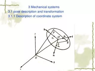
Data description and transformation. What do we look for when we describe univariate data? Peaks/Bumps Location Spread Outliers. Window glass. Patterned Glass. Toughened glass. Borosilicates. Lead glass. Data description. Peaks/Bumps Unimodal Bimodal Multimodal

E N D
Data description and transformation What do we look for when we describe univariate data? Peaks/Bumps Location Spread Outliers Statistical Data Analysis - Lecture 03 - 07/03/03
Window glass Patterned Glass Toughened glass Borosilicates Lead glass Statistical Data Analysis - Lecture 03 - 07/03/03
Data description • Peaks/Bumps • Unimodal • Bimodal • Multimodal Why is there more than one mode? • Contamination • Mixing of more than one process? Statistical Data Analysis - Lecture 03 - 07/03/03
10 8 All Male Female Frequency 6 4 2 155 160 165 170 175 180 185 190 Height in cm Statistical Data Analysis - Lecture 03 - 07/03/03
Outliers • Outliers are: • Abnormal data points – “different from the bulk of the data”. • They may be: • Data entry errors • Measurement errors • Just really different pieces of data • Outliers should always be investigated! Statistical Data Analysis - Lecture 03 - 07/03/03
Symmetry and skewness • Data may also be described in terms of symmetry or skewness • If the extreme values of the data set lie to the left of the mean or median then the data is said to be left skewed. • Conversely, if the extreme values of the data set lie to the right of the mean or median then the data is said to be right skewed. Statistical Data Analysis - Lecture 03 - 07/03/03
Right Skewed/Postively Skewed • Long tail to the right • Bulk of the data to the left of the mean • Mean = 0.20 • Left skewed/Negatively Skewed • Long tail to the left • Bulk of the data to the right of the mean • Mean = 0.93 Statistical Data Analysis - Lecture 03 - 07/03/03
Symmetry takes many different forms Statistical Data Analysis - Lecture 03 - 07/03/03
Summary Statistics • Measures of location • mean • median • Measures of spread • variance/std. deviation • range • interquartile range (IQR) Statistical Data Analysis - Lecture 03 - 07/03/03
Order statistics and quantiles If our data are x1, x2, … , xn then the order statistics are simple the data sorted into ascending order and denoted x(1), x(2), … , x(n) and x(1)x(2) … x(n) If is of the form for some integer i, define the corresponding quantile to be the ith order statistic, i.e. • The quantile, q , is chosen such that approximately 100% of the data is less than q . • For example if = 0.1 then approximately 10% of the data has a value less than the 0.1 quantile q0.1 Statistical Data Analysis - Lecture 03 - 07/03/03
Example • Let x = {9, 6, 10, 5, 3, 1, 5, 5, 10, 6} • Then the order statistics are {1, 3, 5, 5, 5, 6, 6, 9, 10, 10} • The first order statistic x(1) = 1, is the quantile • That is, • The last order statistic is x(10) = 10, is 0.91 quantile • Why isn’t x(10) the 1.0 quantile? • Imagine that we’re finding quantiles for the normal distribution. What is the point x such that Pr(X < x) = 1? • The answer is + (positive infinity). This will cause us problems later on. Statistical Data Analysis - Lecture 03 - 07/03/03
Quantiles • The,0.25 quantile is the lower quartile • The 0.5 quantile is the median • The 0.75 quantile is the upper quartile If you want a quantile from the data that is not represented by any i(e.g. if n = 10, and = 0.1), then it can be interpolated from the data by taking a weighted sum of the two surrounding quantiles Statistical Data Analysis - Lecture 03 - 07/03/03
The Symmetry Statistic • The symmetry statistic provides a numerical summary of symmetry. • It is defined as: “The ratio of the distance from the median to the lower quantile to the interquantile difference” is usually chosen to be 0.1 or 0.05. We will use 0.1 Statistical Data Analysis - Lecture 03 - 07/03/03
The symmetry statistic • If S is less than 0.5 then the data is right skewed • The quantile is closer to the median than the 1 - quantile • If S is greater than 0.5 then the data is left skewed • The 1 - quantile is closer to the median than the quantile Statistical Data Analysis - Lecture 03 - 07/03/03
Transforming data • Sometimes we want to make data more symmetric. Why? • Makes it easier to see what is going on • Meet the assumptions of some parametric test • Makes the data better behaved • How do we transform the data? • Can apply any mathematical function but typically we use power transformations Statistical Data Analysis - Lecture 03 - 07/03/03
Power transformations • Note these only work for positive data • Can raise data to an positive integer or fractional power p, for example p=0.5 (square root) or p = 3 (cubed data). • Or raise data to a negative power – remember x-p = 1/xp. • When p = 0, we use the logarithm. Why? Statistical Data Analysis - Lecture 03 - 07/03/03
Choosing an optimal transformation • In general: • Increasing power (>1) will correct left skew • Decreasing power (<1) will correct right skew • Always choose a transformation you can explain (rounding is a good start) • A log transformation is often all you need • Symmetry power plot • Plot power (p) versus symmetry statistic S Statistical Data Analysis - Lecture 03 - 07/03/03