Download
1 / 28
590 likes | 956 Views
102-1 Under-Graduate Project Case Study: Single-path Delay Feedback FFT. Speaker: Darcy Tsai Advisor: Prof. An- Yeu Wu Date: 2013/10/31. Outline. Introduction of Fast Fourier Transform (FFT) DFT/IDFT & FFT/IFFT Flow Graph of FFT Algorithm Hardware Implementation Radix-n FFT Algorithm

E N D
102-1 Under-Graduate ProjectCase Study: Single-path Delay Feedback FFT Speaker:Darcy Tsai Advisor: Prof. An-Yeu Wu Date: 2013/10/31
Outline • Introduction of Fast Fourier Transform (FFT) • DFT/IDFT & FFT/IFFT • Flow Graph of FFT Algorithm • Hardware Implementation • Radix-n FFT Algorithm • System Design Flow • Floating Point Modeling • Fixed Point Modeling • Simulation
x[n] Time domain sequence X[k] Frequency domain spectrum DFT IDFT Twiddle factor : DFT/IDFT • Definition of Discrete Fourier Transform(DFT) and Inverse DFT(IDFT)
FFT/IFFT • Fast Fourier Transform (FFT) is based on the concept of “Divide-and-Conquer” • The complexity of DFT: N2 • The complexity of FFT: Nlog2N • Decimation-in-Time(DIT) FFT Algorithm —
Flow Graph of DIT FFT Algorithm Pre-processing Post-processing
Flow Graph of DIT FFT Algorithm • Computation: Nlog2N N N N log2N stages
Flow Graph of DIT FFTAlgorithm DFT-4 DFT-2 Bit-reverse order Normal order 000 100 010 110 001 101 011 111 000 001 010 011 100 101 110 111 [1]
Flow Graph of DIF FFTAlgorithm DFT-2 DFT-4 Normal order Bit-reverse order 000 001 010 011 100 101 110 111 000 100 010 110 001 101 011 111 [1]
Reuse of Single Butterfly Hardware Implementation Fully Spread • Slow ————Speed———— Fast Small ————Area ————Large Complex ———— Control ———— Simple
Radix-4 FFT Algorithm • Radix-4: decimation into 4 groups
Radix-2 Single-path Delay Feedback for N=16 Radix-4 Single-path Delay Feedback for N=256 [2]
Radix-n FFT Algorithm • For Radix-n FFT, the complexity is NlognN • Larger N — • Less complex multiplier • Less stages • More complex butterfly structure • Designing at algorithm level outperforms others • Pipeline, Parallel, Retiming, Folding/Unfolding
BF2i BF2ii BF4 Relationship of Radix-4 & Radix-22 [2]
BF2ii BF2i Xr(n) Zr(n+N/2) Xr(n) Zr(n+N/2) 0 0 1 1 Xi(n) Zi(n+N/2) Xi(n) Zi(n+N/2) 0 0 1 1 ± Zr(n) Xr(n+N/2) 0 Zr(n) Xr(n+N/2) - 1 1 - 0 0 1 Xi(n+N/2) 1 Zi(n) Xi(n+N/2) Zi(n) 1 1 - ± 0 0 0 s s t Radix-22 Single-path Delay Feedback for N=256 s t s t s t s t [2]
System Design Flow Physical Model MATLAB Floating Point Model Optimize Fixed Point Model Simulation MATLAB Verilog Verification
Floating Point Model • Implemented with MATLAB / C code • Translate physical structure to high level language • Keep original signal flow intact
Butterfly(16) Butterfly(8) Butterfly(4) Butterfly(2) Floating Point Model -j -j -j -j -j -j -j -j
Fixed Point Model • Simulate truncation due to limited word-length • Dynamic range of input is critical • Ex: Only 3-bit of fractional part 1.422(10) 1.422(10) (floating point) 1.422(10) 1.011011(2) = 1 + 2-2+ 2-3 = 1.375 • Input signal are truncated to limited precision • Apply truncation where arithmetic is applied after the multiplier module • Twiddle factors are also truncated before introduced to multiplier Fixed Point Model of FFT
Fixed Point Model of FFT -j -j -j -j -j -j -j -j
Simulation • Parameterize the word-lengths of input • Integer word-length • Fractional word-length • Twiddle factor word-length • Insert randomly generated floating point input • Compare with floating point result from MATLAB (SQNR computing)
Calculation of SQNR • SQNR: Signal-to-Quantization-NoiseRatio
Optimal set: 2+6 = 8 Integer 2 bits Fractional 6 bits
Optimal set: 9+2 = 11 Integer 2 bits Twiddle 9 bits
Optimal set: 9+7 = 15 Twiddle 9 bits Fractional 7 bits
Verification • Word-lengths chosen: • Integer 2 bits • Fractional 7 bits • Twiddle 9 bits • Run multiple random tests (105 times) to ensure we have desired results • Adjust bit lengths to ensure the SQNR ≧ 50 if necessary
References [1] Alan V.Oppenheim, Ronald W. Schafer, “Discrete-time signal processing” 2nd edition. [2] E.H. Wold and A.M. Despain. “Pipelined and parallel-pipelined FFT processors for VLSI implementation.,” IEEE Trans. Comput., May 1984 [3] Shousheng He and Torkelson, M., “A new approach to pipeline FFT processor,” Proceedings of IPPS '96, 15-19 April 1996, pp766 –770.