Download
1 / 32
710 likes | 1.49k Views
repulsion. attraction. attraction. Electron Correlation. Hartree-Fock results do not agree with experiment. Heirarchy of methods to treat electron-electron interactions electron correlation ie what approximation do we use for H ?. -. -. +.

E N D
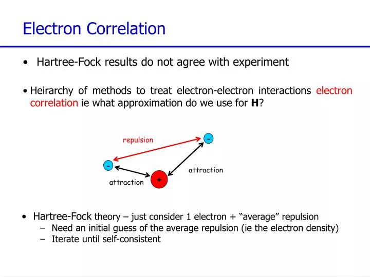
repulsion attraction attraction Electron Correlation • Hartree-Fock results do not agree with experiment • Heirarchy of methods to treat electron-electron interactions electron correlationie what approximation do we use for H? - - + • Hartree-Fock theory – just consider 1 electron + “average” repulsion • Need an initial guess of the average repulsion (ie the electron density) • Iterate until self-consistent
What Tools Can We Use? • Density Functional Theory quantum method in principle “exact” faster than traditional ab initio variable accuracy no systematic improvement Walter Kohn, Nobel Prize 1998
Density Functional Theory The energy and electronic properties of the ground state are uniquely determined by the electron density: E = E[] • In principal this expression is exact! • But we don’t know what the functional is • Use model systems and fitting to derive expressions giving different “functionals” • The electron density is something we can “see” • The electron density is a 3-dimensional property whereas wavefunction-based methods are 3N dimensional • Using the Kohn-Sham orbitals DFT is mathematically equivalent to HF theory
Density Functional Theory ET The kinetic energy EV The Coulomb attraction of the electrons to the nucleus EJThe Coulomb energy of that the electrons would have in their own field, assuming they moved independently and if each electron repelled itself EX The Exchange energy EC The Correlation energy EXC corrects for the false assumptions in EJ
First Generation DFT Energy a functional of r alone Analytic expressions derived from the uniform electron gas Local Density Approximation Local Spin Density Approximation LDA functionals were originally developed for metals and assume the electron density is constant, not a sensible assumption in a molecule. LDA tends to underestimate exchange energies by up to 10%, to overestimate correlation energies by up to a factor of two and to “overbind” molecules. This approximate cancellation of errors made initial LDA results look so promising…
Second Generation DFT Used LDA/uniform electron gas expressions for ET, EV and EJ Invoked the generalised gradient approximation (GGA) for EXC to attempt to correct for non-local interactions, inhomogeneities in the electron gas, using the gradient of the density: Meta functionals incorporate the local kinetic energy density, t(r), which is dependent on the Kohn-Sham orbitals:
Second Generation DFT GGAs, and meta-GGAs are “local” functionals because the electronic energy density at a single spatial point depends only on the behavior of the electronic density and kinetic energy at and near that point. Examples of second generation functionals include Becke’s 1986 exchange functional, the LYP correlation functional, and the PBE and the PW91 functionals These functionals are commonly used in plane wave DFT calculations and in calculations on large systems
Third Generation DFT Functionals where the electronic energy is a functional of the electron density, its gradient and its Laplacian, that is, E[r;r;2r] Hybrid functionals where a proportion of the exact HF exchange energy is included to introduces a degree of “non-local” behaviour The most popular hybrid functional is the B3LYP functional: where the coefficients were found empirically Hybrid functionals generally perform better than GGA functionals in chemical applications
Fourth Generation DFT Meta-hybrid functionals Double hybrid functionals Extensively parametrisedfunctionals…. These functionals attempt to correct for the “local” behaviour of DFT and give much better results for systems with weak or non-bonded interactions
DFT Performance LDA: Works well for anything where the uniform electron gas is a sensible model (eg metals) and for bulk properties Not accurate for chemical applications GGA: Fast Binding energies to about 20 kcal/mol Hybrid functionals: Slower (HF exchange costs) 3-12 kcal/mol errors Fourth generation functionals: Relatively expensive… Claim to do a lot better
Density Functional Theory Density Functional Theory is only marginally more expensive than HF theory. Because it contains an estimate of the electron correlation energy it should always be used in preference to HF HOWEVER, DFT calculations must be validated by comparison against some higher level of theory (sometimes they fail catastrophically…)
Model Chemistries • Theoretical models are defined by specifying a correlation procedure and a basis set • HF/STO-3G: A very simple theoretical model (level of theory) • MP2/6-31G(d): An intermediate level of theory • CCSD(T)/6-311+G(3d,2p): A high level of theory • B3LYP/6-31G(d): A cost effective level of theory • Some properties (eg geometry) can be obtained reliably at simple levels of theory • Others (eg reaction energy, reaction barrier) require a high level of theory
Beyond HF: Electron Correlation Methods • For a given basis set, the difference between the exact energy and the HF energy is the correlation energy, ~ 85 kJ/mol correlation energy per electron pair • Dynamic correlation: electrons repel each other and get out of each other’s way; dynamical motions of electrons are correlated, so electron repulsion is less than in an independent electron model such as HF theory • Static Electron Correlation/Non-Dynamic Electron Correlation/Intrinsic Electron Correlation: arises when a single configurational treatment (ie a single determinant) is not adequate to describe the problem (eg the ground state of the molecule)
Frozen Core Approximation • assume that only the valence electrons are correlated • the core orbitals are treated at the HF level of theory • This assumption is normally good for systems involving first and second row atoms • For third row, or higher, the approximation should probably be checked • for example, if you are not careful in studying a molecule like CaF2, you may find that in the Ca2+ species none of the electrons have been correlated because the 3p orbitals are considered core orbitals (and the F atoms have effectively removed the valence 4s electrons)
Møller-Plesset Perturbation Theory • Although correlation energy is large on a chemical scale it is small compared to the total energy of an atom • We can treat correlation as a perturbation to the HF Hamiltonian • Expand the perturbation in l: • Møller-Plesset perturbation theories, MP2, MP3, MP4… are obtained by setting l=1 and truncating at the 2nd, 3rd, 4th… order terms in l for the wavefunction (l+1 for the energy).
Møller-Plesset Perturbation Theory • Not a variational method • Overcorrection possible • Not appropriate if compound is not well described by a simple Lewis structure • Does not do well in cases of spin contamination • Computational effort nN4 (MP2) n3N4 (MP4) for n electrons and N orbitals • Does not converge smoothly (oscillates) • Sometimes nonconvergent series (eg Ne) • MP2 often gives better results than MP3, MP4…
Configuration Interaction • Mathematically we want to allow electrons in the wavefunction to be able to move together • We can re-expand the wavefunction in terms of some orthogobal basis that encapsulates this concerted movement • We can use all possible HF-SCF determinants as this basis • A determinant describes an electron configuration, “excited” determinants excite one or more electrons into unoccupied orbitals • They are all orthogonal to each other • This single, double, triple etc excitation correlates the electrons
Configuration Interaction • The wavefunction is expanded as a linear combination of all possible HF-SCF determinants • The CI coefficients bs are determined variationally • The size of the FCI calculation depends on the number of electrons, n, and the number of orbitals, N. • For N basis functions there are 2N spinorbitals and the total number of determinants is (2N!)/[n!(2N-n)!] ~ eN
Configuration Interaction • CIS – include all possible single electron excitations:simplest qualitative method for electronic excited states, but not for correlation of the ground state • CISD – include all single and double excitations (yields ~O2V2 determinants)most useful for correlating the ground state • CISDT – singles, doubles and triples (~O3V3 determinants) • Full CI (FCI) – (~((O+V)!/O!V!) determinants) exact for a given basis set O occupied V virtual orbitals
Coupled Cluster Theory • The CI expansion converges slowly • Some excitations are more important than others… • Define a cluster operator:T= 1 + T1 + T2 + T3 +… • Write Y as • Where • This is particularly clever because
Coupled Cluster Theory • If we truncate T T= 1 + T1 + T2 • Then eTwill contain products of T1 and T2 that are equivalent to higher order excitations • T12 represents all double excitations arising from “disconnected” single excitations, • T22 represents all quadruple excitations arising from disconnected double excitations These disconnected excitations turn out to be important (than the generic n-electron excitations) so the coupled cluster wavefunction converges much more rapidly than the CI expansion
CCSD(T) • Truncate T T= 1 + T1 + T2 • Include T3 as a perturbation • Simpler and faster and almost as accurate as CCSDT The CCSD(T) method is the highest level theory available for routine use. With a large basis set CCSD(T) is considered the “Gold Standard” for dynamic electron correlation: CCSD(T)/aug-ccpVTZ
Static Correlation • If the wavefunction is not well described as a single determinant • Species with significant diradical character • Transition States (frequently) • Bond breaking processes • Often for excited electronic states • Unsaturated transition metal complexes • molecules containing atoms with low-lying excited states (Li, Be, transition metals, etc) • along reaction paths in many chemical and photochemical reactions • Generally any species with near degeneracies The T1 diagnostic in CC methods is an indicator of the validity of a single reference approach. T1 > 0.01 casts suspicion on the applicability of single reference methods.
Multi-Configuration Methods • Similar to the CI expansion • Optimise the one-electron orbitals rather than leave them at their HF values • EgMR-CI(SD), CASSCF, CASPT2 … • Starting to get into some serious computational expense…
Cyclobutadiene • 4 p electrons and 4 p molecular orbitals • Each diagram represents a determinant (a configuration state function) • The overall wavefunction is a combination of the possible determinants • The coefficients of the orbitals change with their occupancy (consider square vs rectangular cyclobutadiene)
Cyclobutadiene Active space: 4 electrons in 4 orbitals Core inactive space: remaining 16 electrons in 8 orbitals Virtual/Unoccupied orbitals
Model Chemistries Choosing a method (theoretical model) in ab initio calculations involves striking a compromise between accuracy and computational expense – the more reliable the calculations generally the more computationally demanding The method chosen depends on • The size of the molecule being examined • The property being calculated • The accuracy that is required • The computing resources that are available
Pople Diagram A specific level of theory (theoretical model) corresponds to a combination of correlation procedureand basis set Improvement of Correlation Treatment Full Configuration Interaction HF MP2 MP4 CCSD(T) STO-3G 3-21G 6-31G(d) 6-311+G(2df,p) Improvement of Basis Set Completely Flexible Basis Set Exact Soln of Schrödinger Equation John Pople Nobel Prize 1998 The better you do the longer it takes
Composite Methods • Extrapolate to the bottom right corner of the Pople diagram • Aim is better than 1 cal/mol accuracy • Gaussian “n” methods • G1, G2, G2MP2, G3… • Complete Basis Set Limit (CBS) methods • Weizmann Wn methods • HEAT method…
Summary • Computational chemistry can be used to predict molecular properties, such as: • Equilibrium geometries • Transition structures • Reaction potential energy surfaces • Many tools are available. In general, the more accurate the method the more costly it is to use • Before using a particular approach and methodology, you need to make sure it is accurate enough for your particular problem
Some Observations • Chemists like simple systems • Chemists are interested in electrons so they tend to use the most accurate methods they can • Big problems need to be distilled into small enough bits to provide sensible results • Everything kicks up more questions, nothing is ever as simple as it seems