Download
1 / 23
230 likes | 335 Views
Using Don’t Cares - full_simplify command. Major command in SIS - uses SDC, ODC, XDC Key Questions: How do we represent XDC to a network? How do we relate ODC + XDC to a node representation where ODC is some subset of. full_simplify. y. y. z. XDC. =. z (output). 10. 11. or.

E N D
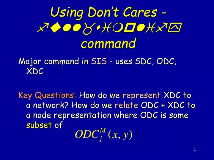
Using Don’t Cares - full_simplify command Major command in SIS - uses SDC, ODC, XDC Key Questions: How do we represent XDC to a network? How do we relate ODC + XDC to a node representation where ODC is some subset of
full_simplify y y z XDC = z (output) 10 11 or y12 separate DC network y9 y2 y1 y10 y11 y5 y6 y3 y4 y7 y8 x1 x3 x2 x4 x1 x3 x4 x1 x2 x4 x2 x3 multi-level Boolean network for z
full_simplify XDC is held in separate network, called the DC network. Described in BLIF by .begin dc ... .end dc XDC and ODC are related only through x1, x2, x3, x4, the primary inputs.
yj yl yr x1 x2 xn Mapping to Local Space How can ODC + XDC be used for optimizing the representation of a node, yj?
Mapping to Local Space Definitions: The local space Br of node j is the Boolean space of all the fanins of node j (plus maybe some other variables chosen selectively). A don’t care set D(yr+) computed in local space (+) is called a local don’t care set. Solution: Map DC(x) = (ODC+XDC)(x) to local space of the node to find local don’t cares, i.e. we will compute
yj yl yr x1 x2 xn Computing Local Don’t Cares The computation is done in two steps: 1. Find DC(x) in terms of primary inputs. 2. Find D, the local don’t care set, by image computation and complementation.
yj yl yr x1 x2 xn Map to Primary Input (PI) Space
Map to Primary Input (PI) Space Computation done with Binary Decision Diagrams • Build BDD’s representing global functions at each node in both the primary network and the don’t care network, gj(x1,...,xn) - use BDD_compose or better, BDD_substitute. • Replace all the intermediate variables in (ODC+XDC) with their global BDD • Since we will be using the method of computing the compatible don’t cares by the “local cube method”, in general, this will be a set of cubes expressed in (x,y) • Use BDD’s to substitute for y in the above (using BDD_substitute) ~ = + ® = h ( x , y ) ( ODC XDC )( x , y ) h ( x ) DC(x)
Example XDC z (output) y12 or separate DC network or y9 y2 y1 & y10 y11 y5 y6 & xnor y3 y4 & y7 y8 & x1 x3 x2 x4 x1 x3 x4 x1 x2 x4 x2 x3 multi-level network for z
local space gr gl yj yl yr x1 x2 xn Image Computation image of care set under mapping y1,...,yr Br Di image Bn DCi=XDCi+ODCi care set • Local don’t cares are the set of minterms in the local space of yi that cannot be reached under any input combination in the care set of yi. • Local don’t Care Set: • i.e. those patterns of (y1,...,yr) that never appear as images of input cares.
XDC z (output) y12 y9 y2 y1 y10 y11 y5 y6 y3 y4 y7 y8 x1 x3 x2 x4 x1 x3 x4 x1 x2 x4 x2 x3 Example or separate DC network or & & xnor & & multi-level network for z Note that D2 is given in this space y5, y6, y7, y8. Thus in the space 2210 never occurs. Can check that Using , f2 can be simplified to
Full_simplify Algorithm • Visit node intopological reverse order i.e. from outputs. This gives rise to a total ordering of all nodes. Edge ordering is inherited from node ordering, i.e. [i,j] < [k,j] if i < k. • Compute compatible ODCi by “modified flipping” method. • compatibility done in SOP form with intermediate y variables. • BDD’s built to get this don’t care set in terms of primary inputs (DCi) • Image computation techniques used to find local don’t cares Di at each node.( XDCi + ODCi )(x,y) DCi(x) Di( y r )where ODCi is a compatible don’t care at node i. f y1 yk
Easier Computation of CODC Subset The Savoj method, an easy way for computing a CODC subset on each input of a function f, is:where CODCf is the compatible don’t cares already computed for node f, and where f has its inputs y1,y2,... in that order.
Image Computation: two methods • Transition Relation Method f : Bn Br F : Bn x Br B F is the characteristic function of f.
Transition Relation Method • Image of set A under f f(A) = x(F(x,y)A(x))The existential quantification x is also called “smoothing” and denoted sometimes by Sx. Note:The result is a BDD representing the image, i.e. f(A) is a BDD with the property that BDD(y) = 1 x such that f(x) = y and x A. f A f(A) x y
Recursive Image Computation Problem:Given f : Bn Br and A(x) Bn Compute: Step 1: compute CONSTRAIN(f,A(x)) fA(x)f and A are represented by BDD’s. CONSTRAIN is a built-in BDD operation. It is related to generalized cofactor with the don’t cares used in a particular way to make 1. the BDD smaller and 2. an image computation into a range computation. Step 2: compute range of fA(x). fA(x) : Bn Br
Recursive Image Computation Property of CONSTRAIN (f,A) fA(x): (fA(x))|xBn = f|xAi.e. range = image f A f(A) fA range of fA(Bn) Bn Br range of f(Bn)
Recursive Image Computation Divide and conquer 1. Bn Br = (y1,...,yr) This is calledinput cofactoring
Recursive Image Computation Divide and conquer 2. where here refers to the CONSTRAIN operator. (This is called output cofactoring). Thus Notes: This is a recursive call. Could use 1. or 2 at any point. The input is a set of BDD’s and the output can be either a set of cubes or a BDD.
BDD_CONSTRAIN illustrated A f 0 0 X X Idea:Map subspace (say cube c in Bn) which is entirely in DC (i.e. A(c) 0) into nearest non-don’t care subspace(i.e. A 0). where PA(x) (projection) is the “nearest” point in Bn such that A = 1 there.
full_simplify XDC outputs fj m intermediate nodes Don’t Care network inputs Bn Express ODC in terms of variables in Bn+m
full_simplify Express ODC in terms of variables in Bn+m Bn Bn+m Br ODC+XDC D DC compose cares cares image computation Minimize fj don’t care = D fj local space Br Question: Where is the SDC coming in and playing a roll?