Download

1 / 20
200 likes | 336 Views
3.2 Linear Programming I. Vertex Fundamental Theorem of Linear Programming Linear Programming Steps. Vertex.

E N D
3.2 Linear Programming I • Vertex • Fundamental Theorem of Linear Programming • Linear Programming Steps
Vertex • The boundary of the feasible set is composed of line segments. The line segments intersect in points, each of which is a corner of the feasible set. Such a corner is called a vertex.
Example Vertex • Find the vertices of • y< -2x + 32 • y< -x + 18 • y< -x/3 + 12 • x> 0, y> 0. (9,9) (0,12) (14,4) (0,0) (16,0)
Fundamental Theorem of Linear Programming • Fundamental Theorem of Linear ProgrammingThe maximum (or minimum) value of the objective function in a linear programming problem is achieved at one of the vertices of the feasible set. The point that yields the maximum (or minimum) value of the objective function is called an optimal point.
Example Optimal Point • Find the point which maximizes Profit = 80x + 70y for the feasible set with vertices (0,0), (0,12), (9,9), (14,4) and (16,0).
Example Linear Programming Steps • Rice and soybeans are to be part of a staple diet. One cup of uncooked rice costs 21 cents and contains 15 g of protein, 810 calories, and 1/9 mg of B2 (riboflavin). One cup of uncooked soybeans costs 14 cents and contains 22.5 g of protein, 270 calories, and 1/3 mg of B2. The minimum daily requirements are 90 g of protein, 1620 calories and 1 mg of B2. Find the optimal point that will minimize cost.
Example Step 1A Organize the data.
Example Step 1B • B. Identify the unknown quantities and define corresponding variables. • x = number of cups of rice per day • y = number of cups of soybeans per day
Example Step 1C • C. Translate the restrictions into linear inequalities. • Protein: 15x + 22.5y> 90 • Calories: 810x + 270y> 1620 • B2: (1/9)x + (1/3)y> 1 • Nonnegative: x> 0, y> 0
Example Step 1D • D. Form the objective function. • Minimize the cost in cents: • [Cost] = 21x + 14y
Example Step 2A • A. Put the inequalities in standard form. • Protein: y> (-2/3)x + 4 • Calories: y> -3x + 6 • B2: y> (-1/3)x + 3 • Nonnegative: x> 0 • y> 0
Example Step 2B 4 2 • B. Graph the straight line corresponding to each inequality. • 1. y = (-2/3)x + 4 • 2. y = -3x + 6 • 3. y = (-1/3)x + 3 • 4. x = 0 • 5. y = 0 1 3 5
Example Step 2C • C. Determine the side of the line. • y> (-2/3)x + 4 • y> -3x + 6 • y> (-1/3)x + 3 • x> 0 • y> 0 feasible set
Example Step 3 • Determine the vertices of the feasible set. • x = 0 & y = -3x + 6: (0,6) • y = -3x + 6 & y = (-2/3)x + 4: • (6/7,24/7) • y = (-2/3)x + 4 & y = (-1/3)x + 3: • (3,2) • y = (-1/3)x + 3 & y = 0: (9,0) (0,6) (6/7,24/7) (3,2) (9,0)
Example Step 4 • Determine the objective function at each vertex. Determine the optimal point. The minimum cost is 66 cents for 6/7 cups of rice and 24/7 cups of soybeans.
Summary Section 3.2 - Part 1 • The fundamental theorem of linear programming states that the optimal value of the objective function for a linear programming problem occurs at a vertex of the feasible set.
Summary Section 3.2 - Part 2 • To solve a linear programming word problem, assign variables to the unknown quantities, translate the restrictions into a system of linear inequalities involving no more than two variables, form a function for the quantity to be optimized, graph the feasible set, evaluate the objective function at each vertex, and identify the vertex that gives the optimal value.