Download
1 / 35
350 likes | 943 Views
Linear Programming. Joseph Mark November 3, 2009. What is Linear Programming. Linear Programming – a management science technique that helps a business allocate the resources it has on hand to make a particular mix of products that will maximize profit.

E N D
Linear Programming Joseph Mark November 3, 2009
What is Linear Programming • Linear Programming – a management science technique that helps a business allocate the resources it has on hand to make a particular mix of products that will maximize profit. • Tool for maximizing or minimizing a quantity subject to constraints • Said to account for 50-90% of computing time used for management decisions
Real World Applications and Examples • What crops to grow on limited farmland • How to use resources in a bakery (eggs, butter, sugar, eggs, flour) • How to use labor force
Linear Programming • Uses an algorithm based on available data to produce an optimal solution • Can take on decimal values unlike integer programming • However, sometimes the optimal solution is an unfeasible solution • It doesn’t make sense to produce 3.24 dolls to sell
Mixture Problem • In a mixture problem, limited resources are combined into products so that the profit from selling those products is a maximum • Example: how different kinds of aviation fuel can be manufactured using different kinds of crude oil • An optimal production policy has two properties. First it is possible; that is, it does not violate any of the limitations under which the manufacturer operates, such as availability of resources. Second, the optimal production policy gives the max profit
Mixture Problems with One Resource • Suppose a toy manufacturer has 60 containers of plastic and wants to make and sell skateboards. • One skateboard requires 5 containers of plastic • The profit on 1 skateboard is $1 • Manufacturer can make 60/5 = 12 skateboards • So the number of skateboards, x, that can be made is between 0 and 12, or 0 ≤ x≤ 12 • These values are the feasible set (set of all possible solutions)
Notes on Feasible Region • Any point within the feasible region represents a possible production policy – any number within this region is possible to produce given the limited supplies. • For most problems, negative values are unfeasible, for example, how do you make negative skateboards? • Maximum profit always occurs at a corner point of a feasible region, in both simple and complex problems
Common Features of Mixture Problems • Resources • Definite resources are available in limited, known quantities for the time period in question. Ex. plastic • Products • Definite products can be made by combining, or mixing, the resources. Ex. Skateboards • Recipes • A recipe for each product specifies how many units of each resource are needed to make one unit of that product. Ex. 1 skateboard = 5 containers of plastic • Profits • Each product earns a known profit per unit • Objective • The objective in a mixture problem is to find out how much of each product to make so to maximize profits without exceeding resource limitations
Two Products and One Resource • Toy manufacturer makes skateboards and dolls • 1 doll requires 2 containers of plastic • 1 skateboard requires 5 containers of plastic • Can make all dolls, all skateboards, or some combination of the two • One doll makes $.55 profit • One skateboard makes $1 profit • Total Profit will be $1x+$.55y, where x is the number of skateboards and y is the number of dolls manufactured
Mixture Charts • Answers • 1. what are the resources • 2. what quantity of each resource is available • 3. what are the products • 4. what are the recipes for the products • 5. what are the unknown quantities • 6. what is the profit formula
Mixture Chart for Skateboards and Dolls RESOURCES Containers of Plastic 60 PROFIT PRODUCTS
Resource Constraints • Tell how much of a resource you have • You can’t use more than the amount available • For the skateboards and dolls problem • The number of plastic containers used must be less than 60 • So 5x + 2y ≤ 60. • Constraint inequalities are always associated with equations for lines, thus linear programming.
Finding the Optimal Production Policy • Now need to find the point within the region that gives the maximum profit • Corner Point Principle • The corner point principle states that in a linear programming problem, the maximum value for the profit formula always corresponds to a corner point of a feasible region
Corner Point Principle • 1. Determine the corner points of the feasible region • 2. Evaluate the profit at each corner point of the feasible region • 3. Choose the corner point with the highest profit as the production policy.
Optimal Production Policy for Skateboards and Dolls • We have three corner points (0, 0) (12, 0) (0, 30) • Evaluate profit formula at these points • $1x + $.55y Maximum profit at (0, 30) = $16.50 This point is called the optimal production policy
Role of Profit Formula • The optimal production policy is dependent on the profit formula. • For example, if the profit for skateboards were $1.05 and profit for dolls were $.40, we would make all skateboards (12,0) instead of all dolls. • However, there may be reasons for wanting to produce both products
Adding Minimums to Mixture Chart RESOURCES Containers of Plastic 60 MINIMUMS PROFIT PRODUCTS
Find New Optimal Solution • Have new corner points at (4,10) (4,20) (8,10) • Can find these points algebraically • (4,10) easy to see • Upper left point has 4 as x-coordinate • Substitute x=4 into second line 5x+2y=60 • 5(4)+2y=60 -> y = 20 • Same for lower right, substitute y=10 instead • 5x+2(10)=60 -> x=8
Finding New Optimal Solution • Substitute new corner points into profit formula • Using profit formula 1: • (4, 10) = 1(4) + .55(10) = $9.50 • (4, 20) = 1(4) + .55(20) = $15.00 • (8, 10) = 1(8) + .55(10) = $13.50 • Using profit formula 2: • (4, 10) = 1.05(4) + .40(10) = $8.20 • (4, 20) = 1.05(4) + .40(20) = $12.20 • (8, 10) = 1.05(8) + .40(10) = $12.40
Summary of Pictorial Method • 1. Identify resources and products • 2. Make a Mixture Chart showing resources, products, recipes for creating products, profit of each product, and the amount of each resource on hand. If problem has minimums, include that as well • 3. Assign unknowns, x or y, to each product. Use the mixture chart to write down the resource constraints, the minimum constraints, and the profit formula • 4. Graph the line corresponding to each resource constraint and determine which side of the line is in the feasible solution (≥ or ≤ ) • 5. Find the corner points and evaluate the profit formula at these points
Mixture Problems with 2 Resources • Consider the toy manufacturer and now has a second constraint of time. • Suppose there are 360 minutes of available labor. • One skateboard requires 15 minutes • One doll requires 18 minutes • Still maintain zero minimum constraints
New Mixture Chart RESOURCES Containers of Plastic 60 Minutes 360 PROFIT PRODUCTS
Resource Constraints • 5x + 2y ≤ 60 containers of plastic • 15x + 18y ≤ 360 minutes available • Profit Formula $1x + $0.55y • Graph two lines and find the intersection
Find New Corner Points • (0,0) (12,0) (0,20) • Find the intersection point • 5x+2y=60 • 15x+18y=360 • Solve for one variable • 18(5x+2y=60) -> 90x+36y=1080 • -2(15x+18y=360) -> -30x-36y=-720 60x = 360 x = 6 5(6)+2y=60 y = 15 (6,15) is last point
Evaluate • Evaluate your new points in your profit formula $1x + $.55y • (0,0) = $0 • (12,0) = 12 + 0 = $12 • (0,20) = 0 + .55(20) = $11 • (6,15) = 6 + .55(15) = $14.25 • So the optimal production policy is to make 6 skateboards and 15 dolls for a profit of $14.25
Mixing Two Juices • A juice manufacturer produces and sells two fruit beverages: Cranapple and Appleberry • 1 gal of Cranapple is 3qts Cranberry Juice and 1qt Apple Juice • 1 gal of Appleberry is 2qts Apple Juice and 2qts Cranberry Juice • Cranapple makes a profit of 2cents/gallon • Appleberry makes a profit of 5cents/gallon
Constraints • You have 200 quarts of Cranberry Juice available and 100 quarts of Apple Juice available, how many gallons of each drink mixture should we make? • Cranberry constraint 3x+2y ≤ 200 • Apple Juice constraint 2x+2y ≤ 100 • X = gallons of cranapple juice • Y = gallons of appleberry juice
With Minimum Constraints • Want x (gallons of cranapple juice) ≥ 20 • Want y (gallons of appleberry juice) ≥ 10 • Get corner points of (20, 10) (20, 40) (50, 25) (60,10) • Evaluate in profit formula 2x+5y • (20,40) is optimal point • But substituting (20,40) into our cranberry juice constraint, we find we only use 3(20)+2(40)=140 of our allotted 200 quarts available. So we have 60 quarts of slack. • So perhaps sell cranberry juice separately or purchase more apple juice if it’s profitable.
Complex Regions • Sometimes there are so many corner points of a feasible region that multiple calculations are needed to determine the coordinates and profits for each one. Computing the profit for every corner point for even the fastest computer could be impossible • Also, it is not possible to visualize the feasible region as a part of two-dimensional space where there are more than two products. Each product is represented by an unknown, and each unknown is represented by a dimension of space. If we have 50 products, we would need 50 dimensions and we couldn’t visualize such a region.
EXCEL • Linear Programming in Excel
Courses for Additional Information • BUAD 361 – Intro to Operations Technology • BUAD 467 – Adv. Data Management & Modeling • MATH 323 – Intro to Operations Research