Download
1 / 47
480 likes | 487 Views
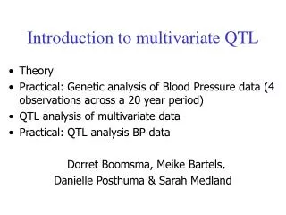
Introduction to multivariate QTL. Theory Practical: Genetic analysis of Blood Pressure data (4 observations across a 20 year period) QTL analysis of multivariate data Practical: QTL analysis BP data Dorret Boomsma, Meike Bartels, Danielle Posthuma & Sarah Medland. Multivariate models.

E N D
Introduction to multivariate QTL • Theory • Practical: Genetic analysis of Blood Pressure data (4 observations across a 20 year period) • QTL analysis of multivariate data • Practical: QTL analysis BP data Dorret Boomsma, Meike Bartels, Danielle Posthuma & Sarah Medland
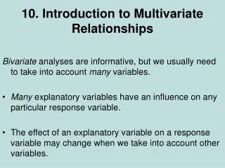
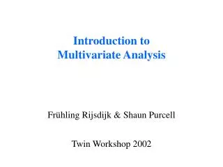
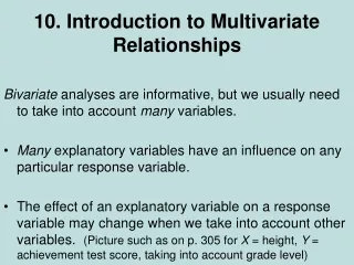
Multivariate models • Principal component analysis (Cholesky) • Exploratory factor analysis (Spss) • Confirmatory factor analysis (Lisrel) • Path analysis (S Wright) • Structural equation models These techniques are used to analyze multivariate data that have been collected in non-experimental designs and often involve latent constructs that are not directly observed. These latent constructs underlie the observed variables and account for correlations between variables.
f 1 2 3 4 x4 x1 x2 x3 e1 e2 e3 e4 The covariance between x1 and x4 is: cov (x1, x4) = 1 4 = cov (1f + e1, 4f + e4 ) where is the variance of f and e1 and e4 are uncorrelated Sometimes x = f + e is referred to as the measurement model. The part of the model that specifies relations among latent factors is the covariance structure model, or the structural equation model
Symbols used in path analysis square box:observed variable (x) circle: latent (unobserved) variable (f) unenclosed variable: disturbance term (error) in equation () or measurement (e) straight arrow: causal relation () curved two-headed arrow: association (r) two straight arrows: feedback loop
Tracing rules of path analysis • The associations between variables in a path diagram is derived by tracing all connecting paths between variables: • 1 trace backward along an arrow, then forward • never forward and then back; • never through adjacent arrow heads • 2 pass through each variable only once • 3 trace through at most one two-way arrow • The expected correlation/covariance between two variables is the product of all coefficients in a chain and summing over all possible chains (assuming no feedback loops)
Genetic Structural Equation Models Confirmatory factor model: x = f + e, where x = observed variables f = (unobserved) factor scores e = unique factor / error = matrix of factor loadings "Univariate" genetic factor model Pj = hGj + e Ej + c Cj , j = 1, ..., n (subjects) where P = measured phenotype G = unmeasured genotypic value C = unmeasured environment common to family members E = unmeasured unique environment = h, c, e (factor loadings/path coefficients)
1 1/.5 C E A E C A a e c a c e P Univariate ACE Model for a Twin Pair rA1A2 = 1 for MZ rA1A2 = 0.5 for DZ Covariance (P1, P2) = a rA1A2 a + c2 rMZ = a2 + c2 rDZ = 0.5 a2 + c2 2(rMZ-rDZ) = a2 P
1/.5 1/.5 A1 A2 A1 A2 a11 a21 a22 a11 a21 a22 P11 P21 P12 P22 e11 e22 e11 e22 e21 e21 E1 E2 E2 E1 Bivariate twin model: The first (latent) additive genetic factor influences P1 and P2; The second additive genetic factor influences P2 only. A1 in twin 1 and A1 twin 2 are correlated; A2 in twin 1 and A2 in twin 2 are correlated (A1 and A2 are uncorrelated)
Identification in Genetics Identification of a genetic model is obtained by using data from genetically related individuals, such as twins, or parents and offspring, and by knowledge about the constraints for certain parameters in the model, whose values are based on Mendelian inheritance. Quantitative genetic theory offers a strong foundation for the application of these models in genetic epidemiology because unambiguous causal relationships can be specified. For example, genes 'cause' a variable like blood pressure and parental genes determine those of children and not vice versa
A C A SY A SX A 1 A 2 hC hC hSX h2 h1 h3 hSY Y1 Y1 X 1 X 1 Bivariate Phenotypes rG A X A Y hX hY Y1 X 1 Cholesky decomposition Correlation Common factor
Correlated factors rG • Genetic correlation rG • Component of phenotypic covariance rXY = hXrGhY +cXrCcY +eXrEeY A X A Y hX hY Y1 X 1
A C A SY A SX hC hC hSX hSY Y1 X 1 Common factor model A constraint on the factor loadings is needed to make this model identified
Cholesky decomposition • If h3 = 0: no genetic influences specific to Y • If h2 = 0: no genetic covariance • The genetic correlation between X and Y = covariance / SD(X)*SD(Y) A 1 A 2 h2 h1 h3 Y1 X 1
1/.5 1/.5 A1 A2 A1 A2 a11 a21 a22 a11 a21 a22 P11 P21 P12 P22 e11 e22 e11 e22 e21 e21 E1 E2 E2 E1 Bivariate twin model: The first (latent) additive genetic factor influences P1 and P2; The second additive genetic factor influences P2 only. A1 in twin 1 and A1 twin 2 are correlated; A2 in twin 1 and A2 in twin 2 are correlated (A1 and A2 are uncorrelated)
Implied covariance structure • See handout
Four variables: blood pressure F1 F2 F3 F4 F: Is there familial (G or C) transmission? P3 P1 P4 P2 E: Is there transmission of non-familial influences? E1 E2 E3 E4
Genome-wide scans for blood pressure in Dutch twins and sibs Phenotypes: Dorret Boomsma (study 1; 1985) Harold Snieder (study 2; 1990) Danielle Posthuma (study 3; 1998) Mireille van den Berg /Nina Kupper (study 4; 2002) Eco de Geus Jouke Jan Hottenga Vrije Universiteit, Amsterdam Genotypes Eline Slagboom Marian Beekman Bas Heijmans Molecular Epidemiology, Leiden Jim Weber Marshfield, USA
Design and N of individuals 56 203 138 N=320 N=424 N=751 N=566 126 14 N of Ss who participated in 3 studies: 53, in 2 studies: 378 and in 1 study: 1146 (only offspring; 1 Ss from triplets and families with size > 6 removed) BP levels corrected for medication use
Study 1 (Dorret): 320 adolescent twins (& parents) • Blood pressure* • Systolic • Diastolic • MAP • Heart rate • Inter-beat interval • Variability • RSA • Pre-ejection period • Height / Weight • Birth size • Non-cholest. Sterols • Lipids • CRP • Fibrinogen • HRG * Assessed in rest and during stress; resting BPaveraged over 6 measures Boomsma, Snieder, de Geus, van Doornen. Heritability of blood pressure increases during mental stress. Twin Res. 1998
Study 2 (Harold): 424 adult twins • Same as study 1 plus • Waist & hip • circumference, • Skin folds • %fat • PAI, • tPA, • v. Willebrand • Glucose • Insuline • Hematocrit BP assessed in rest and during stress; resting BPaveraged over 3 measures Snieder, Doornen van, Boomsma, Developmental genetic trends in blood pressure levels and blood pressure reactivity to stress, in: Behavior Genetic Approaches in Behavioral Medicine, Plenum Press, New York, 1995
Study 3 (Danielle): 751 adult twins and sibs • Cognition • Memory • Executive function • EEG/ ERP • MRI • blood pressure BP assessed in rest; averaged over 3 measures Evans et al. The genetics of coronary heart disease: the contribution of twin studies. Twin Res. 2003
Study 4 (Nina): 566 adult twins and sibs • Ambulatory measures • ECG • ICG • RR • cortisol • blood pressure • Average of at least 3 ambulatory BP measures while sitting (during evening) Kupper, Willemsen, Riese, Posthuma, Boomsma, de Geus. Heritability of daytime ambulatory blood pressure in an extended twin design. Hypertension 2005
Dorret Harold Danielle Nina Sex Variable Study 1 Study 2 Study 3 Study 4 MZ M N 70 92 117 57 age 16.6 (1.8) 42.9 (5.6) 36.8 (12.3) 34.0 (13.1) SBP 119.8 (8.2) 129.1 (11.9) 129.7 (14.4) 129.7 (11.1) DBP 65.6 (6.4) 80.5 (9.6) 77.6 (12.6) 77.5 (9.6) F N 70 98 147 108 age 16.0 (2.2) 45.4 (7.4) 39.0 (13.1) 29.0 (10.5) SBP 115.0 (5.7) 120.7 (12.0) 122.5 (14.4) 124.0 (10.8) DBP 67.6 (4.7) 73.5 (10.0) 74.8 (10.0) 77.1 (9.2) DZ M N 91 114 125 80 age 16.9 (1.8) 44.6 (7.1) 36.2 (13.1) 29.3 (8.8) SBP 119.8 (9.3) 127.6 (11.7) 129.6 (12.4) 131.1 (10.7) DBP 65.6 (7.4) 78.2 (8.9) 77.6 (11.8) 77.6 (8.9) F N 89 120 175 137 age 17.2 (1.9) 44.1 (6.3) 37.0 (12.7) 30.9 (11.3) SBP 115.3 (7.3) 124.5 (16.2) 124.6 (16.2) 125.4 (12.9) DBP 67.9 (5.6) 75.7 (11.8) 76.1 (11.0) 78.0 (10.9) Sib M N - - 88 74 age - - 37.3 (14.2) 35.2 (13.1) SBP - - 128.3 (13.0) 130.4 (9.7) DBP - - 78.3 (11.2) 79.2 (8.4) F N - - 99 110 age - - 37.3 (12.8) 36.7 (11.9) SBP - - 124.3 (16.4) 122.6 (12.2) DBP - - 76.4 (10.2) 77.0 (9.7) Data corrected for medication use (by adding means effect of van anti-hypertensiva)
Stability (correlations SBP / DBP) between measures in 1983, 1990, 1998 and 2003 .57 / .62 .62 / .67 .60 / .59 1983 1990 1998 2003 .51 / .47 .44 / .58 Does heritability change over time? Is heritability different for ambulatory measures? What is the cause of stability over time?
Assignment • ACE Cholesky decomposition on SBP (and / or DBP) on all data (4 time points) • Test for significance of A and C • What are the familial correlations across time (i.e. among A and / or C factors) • Can the lower matrix for A, C, E be reduced to a simpler structure?
Four blood pressure measurements A1 A2 A3 A4 Can A be reduced to 1 factor? BP2 BP3 BP1 BP4 E: Is there transmission over time (is E a diagonal matrix?) E1 E2 E3 E4
A BP1 BP2 BP3 BP4 Can the model for A (additive genetic influences) be reduced to 1 factor?
#DEFINE NVAR 4 #DEFINE NDEF 2 ! NUMBER OF DEFINITION VARIABLES #NGROUPS 3 ! NUMBER OF GROUPS G1: CALCULATION GROUP DATA CALCULATION BEGIN MATRICES X LOWER NVAR NVAR FREE ! ADDTIVE GENETIC Y LOWER NVAR NVAR FREE ! COMMON ENVIRONMENT Z LOWER NVAR NVAR FREE ! UNIQUE ENVIRONMENT H FULL 1 1 FIX ! HALF-MATRIX (contains 0.5) G FULL 1 8 FREE ! GENERAL MEANS SAMPLES R FULL NDEF 1 FREE ! DORRET REGRESSION COEFFICIENTS COVARIATES S FULL NDEF 1 FREE ! HAROLD REGRESSION COEFFICIENTS COVARIATES T FULL NDEF 1 FREE ! DANIELLE REGRESSION COEFFICIENTS U FULL NDEF 1 FREE ! NINA REGRESSION COEFFICIENTS C END MATRICES
G2: MZM DATA NINPUT_VARS=45 MISSING=-99.0000 RECTANGULAR FILE = C11P50.PRN LABELS ID1 ID2 PAIRTP TWZYG DOSEX1 DOAGE1 DOMDBP1 DOMSBP1 DOMED1 HASEX1 HAAGE1 HAMDBP1 HAMSBP1 HAMED1 DASEX1 DAAGE1 DAMDBP1 DAMSBP1 DAMED1 NISEX1 NIAGE1 NIMDBP1 NIMSBP1 NIMED1 DOSEX2 DOAGE2 DOMDBP2 DOMSBP2 DOMED2 HASEX2 HAAGE2 HAMDBP2 HAMSBP2 HAMED2 DASEX2 DAAGE2 DAMDBP2 DAMSBP2 DAMED2 NISEX2 NIAGE2 NIMDBP2 NIMSBP2 NIMED2 PIHAT !data for twin1 and twin2 SELECT IF TWZYG < 4; !MZ Selected SELECT IF TWZYG ^= 2; SELECT DOSEX1 DOAGE1 HASEX1 HAAGE1 DASEX1 DAAGE1 NISEX1 NIAGE1 DOMSBP1 HAMSBP1 DAMSBP1 NIMSBP1 DOSEX2 DOAGE2 HASEX2 HAAGE2 DASEX2 DAAGE2 NISEX2 NIAGE2 DOMSBP2 HAMSBP2 DAMSBP2 NIMSBP2; DEFINITION DOSEX1 DOAGE1 DOSEX2 DOAGE2 HASEX1 HAAGE1 HASEX2 HAAGE2 DASEX1 DAAGE1 DASEX2 DAAGE2 NISEX1 NIAGE1 NISEX2 NIAGE2;
Data and scripts • F:\meike\BP2005\phenotypic • ACEBP Elower.mx: 4 variate script for genetic analysis (Cholesky decomposition) • Input file = C11P50.prn • ACE Cholesky decomposition on SBP (and / or DBP) on all data (4 time points) • Test for significance of A and C • What are the familial correlations across time (i.e. among A and / or C factors) • Can the lower matrix for A, C, E be reduced to a simpler structure?
Stability (correlations SBP / DBP) between measures in 1983, 1990, 1998 and 2003 .57 / .62 .62 / .67 .60 / .59 1983 1990 1998 2003 .51 / .47 .44 / .58 Does heritability change over time? Is heritability different for ambulatory measures? What is the cause of stability over time?
Full Cholesky: standardized matrices MATRIX K This is a computed FULL matrix of order 4 by 4 [=\STND(A)] 1 2 3 4 1 1.0000 0.8813 0.9653 0.9975 2 0.8813 1.0000 0.8873 0.8890 3 0.9653 0.8873 1.0000 0.9814 4 0.9975 0.8890 0.9814 1.0000 MATRIX L This is a computed FULL matrix of order 4 by 4 [=\STND(C)] 1 2 3 4 1 1.0000 1.0000 -0.9999 1.0000 2 1.0000 1.0000 -0.9999 1.0000 3 -0.9999 -0.9999 1.0000 -1.0000 4 1.0000 1.0000 -1.0000 1.0000 MATRIX M This is a computed FULL matrix of order 4 by 4 [=\STND(E)] 1 2 3 4 1 1.0000 -0.0732 0.1795 0.3984 2 -0.0732 1.0000 0.1898 -0.0273 3 0.1795 0.1898 1.0000 0.1498 4 0.3984 -0.0273 0.1498 1.0000 Heritability = 51, 41, 57, 43% Common E = 06, 00, 00, 01% Unique E = 42, 58, 43, 55%
Results total sample (systolic BP) -2log-likelihood of data • ACE Cholesky, 42 parameters, 16261.760 • E diagonal, 36 parameters, 16268.885 • A factor, no C, E Cholesky, 26 parameters, 16263.931 • A factor, no C, E diagonal, 20 parameters, 16270.30
A BP1 BP2 BP3 BP4 The model for A (additive genetic influences) can be reduced to 1 factor. E is both unique to an individual and to an occasion. e1 e2 e3 e4
Reduced model – sex and age regression SPECIFY B DOSEX1 DOAGE1; SPECIFY D HASEX1 HAAGE1; SPECIFY F DASEX1 DAAGE1; SPECIFY K NISEX1 NIAGE1; SPECIFY L DOSEX2 DOAGE2; SPECIFY M HASEX2 HAAGE2; SPECIFY N DASEX2 DAAGE2; SPECIFY O NISEX2 NIAGE2; BEGIN ALGEBRA; J = B*R | D*S | F*T | K*U | L*R | M*S | N*T | O*U; END ALGEBRA; MEANS G+J; MATRIX R This is a FULL matrix of order 2 by 1 1 1 -3.7860 2 0.7127 MATRIX S This is a FULL matrix of order 2 by 1 1 1 -7.2228 2 0.2610 MATRIX T This is a FULL matrix of order 2 by 1 1 1 -6.3103 2 0.5559 MATRIX U This is a FULL matrix of order 2 by 1 1 1 -5.9046 2 0.2267 MATRIX G This is a FULL matrix of order 1 by 8 1 2 3 4 5 6 7 8 110.6834 124.7202 116.1748 128.0688 110.6834 124.7202 116.1748 128.0688
Multivariate QTL effects Martin N, Boomsma DI, Machin G, A twin-pronged attack on complex traits, Nature Genet, 17, 387-391, 1997 See: www.tweelingenregister.org
Multivariate phenotypes & multiple QTL effects For the QTL effect, multiple orthogonal factors can be defined (triangular matrix). By permitting the maximum number of factors that can be resolved by the data, it is theoretically possible to detect effects of multiple QTLs that are linked to a marker (Vogler et al. Genet Epid 1997) For example: on chromosome 19: apolipoprotein E, C1, C4 and C2
Multivariate phenotypes & QTL analysis • Multivariate QTL analysis • Insight into etiology of genetic associations (pathways) • Practical considerations (e.g. longitudinal data) • Increase in statistical power: • Boomsma DI, Using multivariate genetic modeling to detect pleiotropic quantitative trait loci, Behav Genet, 26, 161-166, 1996 • Boomsma DI, Dolan CV, A comparison of power to detect a QTL in sib-pair data using multivariate phenotypes, mean phenotypes, and factor-scores, Behav Genet, 28, 329-340, 1998 • Evans DM. The power of multivariate quantitative-trait loci linkage analysis is influenced by the correlation between variables. Am J Hum Genet. 2002, 1599-602 • Marlow et al. Use of multivariate linkage analysis for dissection of a complex cognitive trait. Am J Hum Genet. 2003, 561-70
Genome-wide scan in DZ twins and sibs • 688 short tandem repeats (autosomal) combined from two scans of 370 and 400 markers for ~1100 individuals (including 296 parents; ~100 Ss participated in both scans) • Average spacing ~8.8 cM (9.7 Marshfield, 7.8 Leiden) • Average genotyping success rate ~85%
Genome-wide scan in DZ twins and sibs • Marker-data: calculate proportion alleles shared identical-by-decent (π) • π = π1/2 + π2 • IBD estimates obtained from Merlin • Decode genetic map • Quality controls: • MZ twins tested • Check relationships (GRR) • Mendel checks (Pedstats / Unknown) • Unlikely double recombinants (Merlin)
A Q For MZ twins: r (A1,A2) = 1 r (Q1,Q2) = 1 For DZ twins and sibs: r (A1,A2) = 0.5 r (Q1,Q2) = “pihat” BP1 BP2 BP3 BP4 e e e e
Assignment chromosome 11 genome scan Marker data: 2 cM spacing Phenotypes in MZ twins and genotyped sib/DZ pairs Model: A factor (4 x 1) Q factor (4 x 1) E diagonal (4 x 4) Script: F:\meike\BP2005\linkage\ reduced model.mx Change script and add QTL (e.g. if C is not needed in the model change the ACE model into AQE) Data: F:\meike\BP2005\Data files chromosoom11 C11Pxx.prn (a different file for every position)
Alpha1-antitrypsin: genotypes at the protease inhibitor (Pi) locus and blood pressure: Dutch parents of twins (solid lines: 130/116 MM males/females, dashed lines 16/22 MZ/MS males/females). Non-MM genotypes have lower BP and lower BP response.
Alpha1-antitrypsin: genotypes at the protease inhibitor (Pi) locus and blood pressure: Australian twins (solid lines: 130/127 MM males/females, dashed lines 23/35 MZ/MS males/females). Non-MM males have lower BP.