Download
1 / 74
760 likes | 783 Views
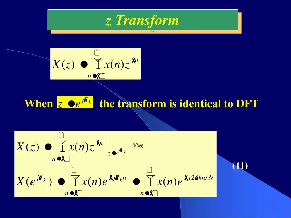
z Transform. When the transform is identical to DFT. (11). z Transform. The sequence x ( n ) is non-zero within [0, N -1], hence. (12). The transform is identical to DFT. Some basic properties of z Transform. 1. Basic definition. 2. Linearity. 3. Delay. 4. Convolution.

E N D
z Transform When the transform is identical to DFT (11)
z Transform The sequence x(n) is non-zero within [0,N-1], hence (12) The transform is identical to DFT
Some basic properties of z Transform 1. Basic definition 2. Linearity 3. Delay 4. Convolution
Essential properties of z Transform 5. Multiplication by ‘z-1’ 6. Relation between X(z) and X(-z) 7. Relation between X(z) and X(z-1)
Why z Transform? 1. z transform can be used to calculate DFT. 2. Filter architecture can be deduced directly from the transfer function in the z domain. Specify filter characteristics (LP, HP, BP...) Determine transfer function H(z) Determine filter sturcture Filter structure can be inferred from H(z) Figure 21
NF M Sbk z-kx(n) y(n)= Sak z-ky(n) + (14) k= -NF k=1 Generalised finite order LTI system NF M Sbk x(n-k) y(n) = Sak y(n-k) + (13) k=1 k= -NF Making use of the delay property, equation (4) can be rewritten as
NF M Sbk z-kx(n) y(n)= Sak z-ky(n) + (14) k= -NF k=1 b-NF z x(n) y(n) b0 + + z-1 z-1 a1 bNF z-1 aM Figure 22
NF M Sbk z-kx(n) y(n) = Sak z-ky(n) + (14) k= -NF k=1 z transform NF M Sbk z-kX(z) Y(z) = Sak z-kY(z) + (15) k= -NF k=1 Note the similarity between the time and z domain
NF M Sbk z-kX(z) Y(z) = Sak z-kY(z) + k= -NF k=1 Digital Filter Design Specify filter characteristics (LP, HP, BP...) Determine transfer function H(z) Rarrange H(z) to the form Construct filter sturcture Figure 21
Example x(n) y(n) + + b0 z-1 z-1 a1 b1 z-1 Figure 23 a2
Poles and Zeros of Transfer Function = (16) Poles and zeros are values of ‘z’ which results in H(z) = infinity and zero, respectively H(z) can be divided into 3 groups for NF > 0 : 1. 2. 3.
Poles and Zeros of Transfer Function Gourp 1 NF poles at z = and NF zeros at z = 0 a zero at z = ckand a pole at z = 0 for each term from k=1 to NP+NF Gourp 2 a zero at z =0and a pole at z = dk for each term from k=1 to M Gourp 3
Example The transfer function can be expressed as Term Group Pole Zero z 1 0 2 0 c1 2 0 c2
Is a filter useful? A filter transfer function H(z) is only useful if : 1. It is stable 2. It is finite
Stability of Transfer Function Given a system with unit-sample response h(n) = [h(0), h(1), ....., h(N-1)] with z transform given by H(z). The system is stable if (17) Finite sequence is generally stable as the absolute sum of finite sample values is always finite
Example The system is unstable
Stability of Transfer Function Generalized LTI transfer function is < for finite NP and NF The numerator The denominator can lead to unstability
Stability of Transfer Function Stability of a digital system depends on the pole locations that are contained in after partial fraction decomposition It can be easily shown that
Stability of Transfer Function For a stable system, For finite summation result, |dk| < 1.
Stability of Transfer Function For a stable system, For finite summation result, |dk| < 1. dk are the poles of H’(z)
Stability of Transfer Function For a stable system, For finite summation result, |dk| < 1. dk are the poles of H’(z) |dk| < 1 means that the poles of a stable system must lies within the unit circle in the z plane.
Region of Convergence (ROC) of Transfer Function A transfer function H(z) is only useful if it is finite, i.e.,
Two classes of digital filters 1. Finite Impulse Response (FIR) Filter 2. Infinite Impulse Response (IIR) Filter The generalised finite order LTI system NF M Sbk x(n-k) y(n) = Sak y(n-k) + (13) k=1 k= -NF formulates an IIR filter
Two classes of digital filters When ak = 0 for all values of k, N-1 Sbk x(n-k) y(n) = (18) k= 0 formulates an FIR filter h(n) = [h(0), h(1), ....., h(N-1)] = [b0, b1, .......bN-1] As N is finite, according to eqn. (17), FIR filter is inherently stable
FIR filters z-1 z-1 z-1 x(n) Figure 24 h(0) h(1) h(2) h(N-1) y(n) (19)
FIR filters Finite Impulse Response (FIR) Filter can guarantee linear phase With linear phase, all input sinsuoidal components are delayed by the same amount. Consider In the frequency domain, Phase delay for frequency w = kw
Phase Distortion - example Given: and (a linear phase X-function) According to previous analysis, (Same signal as before, only delay added to each sample)
Phase Distortion - example Given: and (a non-linear phase X-function) y(n) is not the same as x1(n)
Designing FIR filters from Analogue Transfer Function Analogue Transfer Function H(s) Inverse Fourier Transform h(t) Sample Impulse Response h[n] Corresponding Transfer Function H(z) H(z) = H(s)?
h(t) t Analog to Digital Filters Analogue filter: y(t) = x(t) * h(t) Y(s) = X(s)H(s)
h(t) t 1 unit Analog to Digital Filters Analogue filter: y(t) = x(t) * h(t) Y(s) = X(s)H(s) Given Applying inverse Laplace Transform
h(t) t 1 unit Analog to Digital Filters Digital filter: Sampled and Digitized x(t) and h(t) x(t) -> x(n) , h(t) -> h(n) y(n) = x(n) * h(n) Y(z) = X(z)H(z)
Relation between h(n) and H(z) If h(t) is sampled at unit interval, we have h(t) h(t) = e-an for t > 0 t 1 unit
Relation between h(n) , Ts , and H(z) However, h(t) is sampled at interval of TS instead of the following, h(t) t 1 unit Does sampling rate affects the above transfer function?
h(t) t TS unit Relation between h(n) , Ts , and H(z) If h(t) is sampled at interval of TS, 1. h(n) will be replace with h(nTS) 2. Frequency will be scaled by 1/TS Answer this question by computing the transfer function again based on the new sampling rate
h(t) t TS unit Relation between h(n) , Ts , and H(z) If h(t) is sampled at interval of TS, 1. h(n) will be replace with h(nTS) 2. Frequency will be scaled by 1/TS
h(t) t TS unit Relation between h(n) , Ts , and H(z) If h(t) is sampled at interval of TS, 1. h(n) will be replace with h(nTS) 2. Frequency will be scaled by 1/TS
h(t) t TS unit Relation between h(n) , Ts , and H(z) If h(t) is sampled at interval of TS, 1. h(n) will be replace with h(nTS) 2. Frequency will be scaled by 1/TS The transfer function has similar form as before, may not need to re-compute the transfer function again.
Impulse Invariant Given (sampling period of 1 unit) If sampling period changes to TS , then
How good is the method? Suppose Represents the analogue transfer function. If the analogue unit response is sampled by a period TS , Is the digital response similar to the analogue response?
How good is the method? Suppose Represents the analogue transfer function. If the analogue unit response is sampled by a period TS , (a single spectrum becomes an infinite string of replicas) Digital and Analogue responses are equal if the maximum frequency of the signal is restricted to (otherwise the images start to overlap each other)
A Generic Approach in designing FIR filters Given a desire response HD(w), find hD(n) Applying inverse Fourier Transform, we have, (20) Noted that: n is extended to These kind of filter is not available in practice
with n being infinite and assuming Impulse Invariant, the digital transfer function will be identical to the Analogue ones. In practice, the FIR structure in figure 24 cannot be infinite, hence n is restricted by a window function wR(n) (21) (22) circular convolution
Window Functions Rectangular Window Hanning Window Hamming Window Blackman Window
Window Functions Analogue Transfer Function H(s) Inverse Fourier Transform h(t) Sample Impulse Response h[n] Assume Impulse Invariant Apply window function w[n]h[n] Modified Transfer Function H’(z)
|H(w)| Without window -wc wc p -p 0 |H(w)| With window Side lobes -wc wc p -p 0 Effects of Window Functions Consider a low pass response H(s)
A |H(w)| -wc wc p -p 0 Effects of Window Functions 1. Side lobes decreases stop band attenuation A 2. Window determines the length of the FIR filter
|H(w)| Transition Width (TW) wS wP 0 Actual Pass Band Edge Frequency Desired Pass Band Edge Frequency Stop Band Edge Frequency Low Pass FIR Filter Design Consider a Low Pass Frequency Response
Window N A (dB) Rectangular 21 z-1 z-1 z-1 x(n) Hanning 44 Hamming 55 h(0) h(1) h(2) h(N-1) Blackman 75 fs is the sampling frequency y(n) Low Pass FIR Filter Design Relations between the Window, Filter length and A