Appendix I –Z - Transform and Laplace Transform

1. Appendix I –Z-Transform and Laplace Transform Leonard Kleinrock, Queueing Systems, Volume 1: Theory Nelson Fonseca, State University of Campinas

2. I.1 Why Transforms? • They greatly simplify the calculations • They arise naturally in the formulation and the solution of systems problems • Oftentimes they are the only tools we have available for proceeding with the solution at all

3. g f SYSTEM • System: a mapping between the input function and the output function. The system operates on function f to produce the function g. • The f and g functions depend upon an independent time parameter t: f(t) and g(t)

4. Linear time-invariant systems: transforms do appear naturally • Linear system: where a and b are time independent variables • Time-invariant systems • Which functions of time f(t) may pass through our linear time-invariant systems with no change in form? where H is some scalar multiplier

5. These functions are the “eingenfunctions” or “characteristic functions” • Answer: Complex exponential function where s is a complex variable • From the time-invariance property we must have:

6. H is independent of t but may certainly be a function of s • Wish: be able to decompose the function f(t) into a sum (or integral) of complex exponentials, each of which contributes to the overall output g(t) through a computation of the form given: The overall output may be found by summing (integrating) these individual components of the output

7. The Transform Method : decompose our input into sums of exponentials, compute the response to each from these exponentials, and then reconstitute the output from sums of exponentials • Linear time-invariant systems: constant-coefficient linear differential equations

8. Discrete-Time Systems • Discrete Time Systems: the function f is defined in some points, multiples of a unit t where n = …, -2, -1, 0, 1, 2, … • Notation: • For discrete-time systems we still have:

9. Eingenfunctions • H  how much of a given complex exponential we get out of our linear system when we insert a unit amount of that exponential at the input  system (or transfer) function

10. Definition: Kronecker delta function (or unit function)

11. Let us make the change of variable for the sum on the right-hand side of expression, giving:

13. I.2 The Z-Transform

14. The disk |Z| < 1 represents a range of analyticity for F(Z) is the sum of is finite

16. Z-Transform properties

17. Inspection method to find the sequence given the Z-Transform • Look for terms that are easily invertible

18. It is necessary to divide the denominator into the numerator until the remainder is lower degree than the denominator • Example:

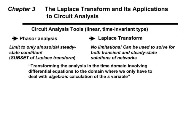
21. I.3 The Laplace Transform • Continuous time • F(t) = 0, t < 0 • Transform a time function in another variable and then “untransform” • For the reasons of invariance of the solution, the “tag” is • Complex variable

22. This Laplace transform will exist so long as f(t) grows no faster than an exponential

23. Region of analyticity Re (s) >= 0 • The properties for the Z-transform when Z=1 will correspond to properties for the Laplace transform when s=0

24. A special case of our one sided exponential function when A=1, a=0 • Definition: • Function with area=1 and value >0, only with t=0

25. 8 a=8 4 a=4 2 a=2 1 a=1 t A -1/2 -1/4 -1/8 -1/16 0 1/16 1/8 1/4 1/2 0 a • As a increases, we note that the pulse gets taller and narrower. The impulse function is defined when a

26. The “derivative” of the unit step function must therefore be a unit impulse function • Sifting property • Derivative of the unit impulse: unit doublet • Function is 0 everywhere, except in the vicinity of the origin it runs off to infinity just to the left of the origin and off to - infinity just to the right of the origin, and, in addition, has a total area equal to zero

27. We can define • Inverse process of the integral

28. Transform of the convolution • Convolution definition:

30. The inspection method for inverse transforms

34. I.4 Use of transforms in the solution of difference and differential equations • Solution of a differential equation Let us consider:

35. Homogeneous and a particular solution: • Homogeneous solution: • General form of solution: where A and aare yet to be determined If we substitute the general solution into the equation, we find:

36. Nth-order polynomial has N solutions: • Associated with each such solution is an which will be determined from the initial conditions (N conditions) • By canceling the common term then the solution is: • Solution: resolution of polynomial equation

37. If there are no multiple roots, the homogenious solution is: • In case of non-distinct roots, the k equal roots will contribute to the following form: • Particular solution: guess from the form of Example:

38. Second-order equation: exist for n=2, 3, 4, …There are two initial conditions, • Homogeneous solution: • Particular solution: must be guessed from

39. Using the initial conditions, we find that

40. Method of Z-transform for solving difference equations • Our approach begins by defining the Z-transform • Then we may apply our inversion techniques • Put G(Z) in evidence and the function is calculated by the inspection method Equation:

43. Solution of constant-coefficient linear differential equations • Solution = homogeneous + particular • The form of the homogeneous solution will be:

47. Solution of differential equations by the Laplace transform