Download
1 / 21

E N D
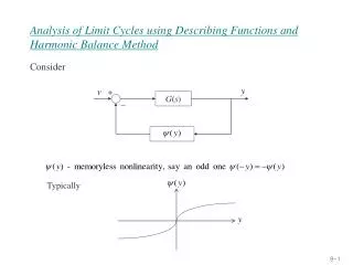
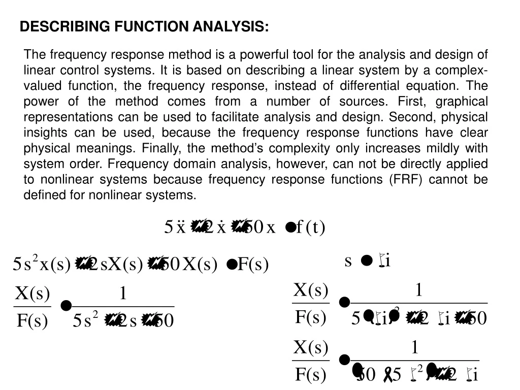
DESCRIBING FUNCTION ANALYSIS: The frequency response method is a powerful tool for the analysis and design of linear control systems. It is based on describing a linear system by a complex-valued function, the frequency response, instead of differential equation. The power of the method comes from a number of sources. First, graphical representations can be used to facilitate analysis and design. Second, physical insights can be used, because the frequency response functions have clear physical meanings. Finally, the method’s complexity only increases mildly with system order. Frequency domain analysis, however, can not be directly applied to nonlinear systems because frequency response functions (FRF) cannot be defined for nonlinear systems.
Using MATLAB Im ϕ Re Phase angle is determined according to the quadrant
clc;clear w=0:0.01:15; s=w*i; Gs=1./(5*s.^2+2*s+50); subplot(211) plot(w,abs(Gs)) title('Frequency Response Function') xlabel('\omega') ylabel('G(\omegai)') grid on subplot(212) plot(w,angle(Gs)*180/pi) xlabel('\omega') ylabel('Phase Angle \phi (Degree)') grid on clc;clear w=0:0.01:15; r=(50-5*w.^2)./((50-5*w.^2).^2+4*w.^2); img=(2*w)./((50-5*w.^2).^2+4*w.^2); Gs=r-img*i; subplot(211) plot(w,abs(Gs)) title('Frequency Response Function') xlabel('\omega') ylabel('G(\omegai)') grid on subplot(212) plot(w,angle(Gs)*180/pi) xlabel('\omega') ylabel('Phase Angle \phi (Degree)') grid on
For some nonlinear systems, an extended version of the frequency response method, called the describing function method, can be used to approximately analyze and predict nonlinear behavior. Even though it is only an approximation method, the desirable properties it inherits from the frequency response method, and the shortage of other systematic tools for nonlinear system analysis, make it an indispensable component of the bag of tools of practicing control engineers. The main use of describing function method is for the prediction of limit cycles in nonlinear systems. An Example of Describing Function Analysis: In this example, we will determine whether there exists a limit cycle in this system and, if so, calculate the amplitude and frequency of the limit cycle (assuming that we have not seen the phase portrait of the Van der Pol equation). where α is a constant. We can represent the system dynamics in a block diagram form, as shown in Figure 1. It is seen that the feedback system contains a linear block and a nonlinear block, where the linear block, although unstable, has low pass properties. Slotine and Li, Applied Nonlinear Control
Linear Element Linear Element s s 0 + 0 + - x - x x x w w - - (.)2 (.)2 =1 =1 Linear element has low pass behavior Figure 1. Feedback interpretation of the Van der Pol oscillator. Linear element is unstable Slotine and Li, Applied Nonlinear Control
Let us assume that there is a limit cycle in the system and the oscillation signal x is in the form of with A being the limit cycle amplitude and ω being the frequency. Thus, Therfore, the output of the nonlinear block is Slotine and Li, Applied Nonlinear Control
Linear Element 0 + x - x w - It is seen that w contains a third harmonic term. Since the linear block has low-pass propertiee, we can reasonably assume that this third harmonic term is sufficiently attenuated by the linear block and its effect is not presented in the signal flow after the linear block. This means that we can approximate w by so that the nonlinear block in Figure 1 can be approximated by the equivalent “quasi-linear” block in Figure 2. The “transfer function” of the quasi-linear block depends on the signal amplitude A, unlike a linear system transfer function (which is independent of the input magnitude). Figure 2. Quasi-linear approximation of the Van der Pol oscillator.
Linear part In the frequency domain, this corresponds to That is, the nonlinear block can be approximated by the frequency response function N(A,ω). Since the system is assumed to contain a sinusoidal oscillation, we have w where G(ωi) is the linear component transfer function. This implies that Denominator Slotine and Li, Applied Nonlinear Control
Solving this equation, we obtain A=2 and ω=1 Note that in terms of the Laplace variable s=ωi, the closed loop characteristic equation of this system is whose roots are Slotine and Li, Applied Nonlinear Control
Corresponding to A=2, we obtain the eigenvalues s1,2=±i. This indicates the existence of a limit cycle of amplitude 2 and frequency 1. It is interesting to note neither the amplitude nor the frequency obtained above depends on the parameter α. α=0.1 α=0.1 α=1 α=1 α=2 α=2 α=4 α=4 In the phase plane, the above approximate analysis suggests that the limit cycle is a circle of radius 2, regardless of the value of α. To verify the plausibility of this result, the real limit cycles corresponding to the different values of α are plotted in Figure 3. It is seen that the above approximation is reasonable for small value of α, but that the inaccuracy grows as α increases. This is understandable because as α grows the nonlinearity becomes more significant and the quasi-linear approximation becomes less accurate. Figure 3. Real limit cycle on the phase plane.
Linear element Nonlinear element w(t) y(t) x(t) r(t)=0 + G(s) w=f(x) - Figure 4. A nonlinear system. Note that, in the approximate analysis, the critical step is to replace the nonlinear block by the quasi-linear block which has the frequency response function (A2/4)(ωi). Afterwords, the amplitude and frequency of the limit cycle can be determined from 1+G(ωi)N(A, ω)=0. The function N(A,ω) is called the describing function of the nonlinear element. The above approximate analysis can be extended to predict limit cycles in other nonlinear systems which can be represented into the block diagram similar to Figure 1. APPLICATIONS OF DESCRIBING FUNCTIONS (DF): Simply speaking, any system which can be transformed into the configuration in Figure 4 can be studied using describing functions. There are at least two important classes of systems in this category. Slotine and Li, Applied Nonlinear Control Slotine and Li, Applied Nonlinear Control
Dead zone and saturation x(t) w(t) u(t) y(t) r(t)=0 + Gp(s) G1(s) - G2(s) Figure 5. A control system with hard nonlinearity. The first important class consists of “almost” linear systems. By “almost” linear systems, we refer to systems which contain hard nonlinearities in the control loop but are otherwise linear. Such systems arise when a control system is designed using linear control but its implementation involves hard nonlinearities, such as motor saturation, actuator or sensor dead-zones, Coulomb friction, or hysteresis in the plant. An example is shown in Figure 5, which involves hard nonlinearitie in the actuator. Consider the control system shown in Figure 5. The plant is linear and the controller is also linear. However, the actuator involves a hard nonlinearity. This system can be rearranged as shown in Figure 4 by regarding GpG1G2 as the linear component G, and the actuator nonlinearity as the nonlinear element. Slotine and Li, Applied Nonlinear Control
“Almost” linear systems involving sensor or plant nonlinearities can be similarly rearranged into the form of Figure 4. The second class of systems consists of genuinely nonlinear systems whose dynamic equations can actually be rearranged into the form of Figure 4. We saw an example of such systems in the previous example (Van der Pol equation). For systems such as the one in Figure 5, limit cycles can often occur due to the nonlinearity. However, linear control cannot predict such problems. Describing functions, on the other hand, can be conveniently used to discover the existence of limit cycles and determine their stability, regardless of whether the nonlinearity is “hard” or “soft”. The applicability to limit cycle analysis is due to the fact that the form of the signals in a limit-cycling system is usually approximately sinusoidal. Indeed, assume that the linear element in Figure 4 has low-pass properties (which is the case of most physical systems). If there is a limit cycle in the system, then the system signals must all be periodic. Since, as a periodic signal, the input to the linear element in Figure 4 can be expanded as the sum of many harmonics, and since the linear element, because of its low-pass property, filters out higher frequency signals, the output y(t) must be composed mostly of the lowest harmonics. Slotine and Li, Applied Nonlinear Control
Prediction of limit cycles is very important, because limit cycles can occur frequently in physical nonlinear system. Sometimes, a limit cycle can be desirable. This is the case of limit cycles in the electronic oscillators used in laboratories. Another example is the so-called dither technique which can be used to minimize the negative effects of Coulomb friction in mechanical systems. In most control systems, however, limit cycles are undesirable. This may be due to a number of reasons: • Limit cycle, as a way of instability, tends to cause poor control accuracy • The constant oscillation associated with the limit cycle can cause increasing wear or even mechanical failure of the control system hardware • Limit cycling may also cause other undesirable effects, such as passenger discomfort in an aircraft under autopilot. In general, although a precise knowledge of the waveform of a limit cycle is usually not mondatory, the knowledge of the limit cycle’s existence, as well as that of its approximate amplitude and frequency, is critical. The describing function method can be used for this purpose. It can also guide the design of compensators so as to avoid limit cycles. Slotine and Li, Applied Nonlinear Control
Basic Assumptions in Describing Function Analysis: • Consider a nonlinear system in the general form of Figure 4. In order to develop the basic version of the describing function method, the system has to satisfy the following four conditions: • Ther is only a single nonlinear components • The nonlinear component is time invariant (saturation, backlash, Coulomb friction, etc.) • Corresponding to a sinusoidal input x=sin(ωt), only the fundamental component w1(t) in the output w(t) has to be considered. • The nonlinearity is odd (symmetry about the origin). w x Saturation Slotine and Li, Applied Nonlinear Control
N.L. N(A,ω) Basic Definitions: Let us now discuss how to represent a nonlinear component by a describing function. Let us consider a sinusoidal input to the nonlinear element, of amplitude A and frequency ω, i.e., x(t)=Asin(ωt) as shown in Figure 6. Figure 6. A nonlinear element and its describing function representation The output of a nonlinear component w(t) is often a periodic, though generally non-sinusoidal, function. Note that this is always the case if the nonlinearity f(x) is single-valued, because the output is f[Asin(w(t+2p/ω))]=f[Asin(ωt)].
Using Fourier series, the periodic function w(t) can be expanded as where the Fourier coefficients ai’s and bi’s are generally functions of A and ω, determined by Slotine and Li, Applied Nonlinear Control
Due to the fourth assumtion above, one as a0=0. Furthermore, the third assumption implies that we only need to consider the fundamental component w1(t), namely where Expression for w(t) indicates that the fundamental component corresponding to a sinusoidal input is a sinusoid at the same frequency. In complex representation, this sinusoid can be written as Slotine and Li, Applied Nonlinear Control
Similarly to the concept of frequency response function, which is the frequency-domain ratio of the sinusoidal input and the sinusoidal output of a system, we define the describing function of the nonlinear element to be the complex ratio of the fundamental component of the nonlinear element by the input sinusoid, i.e., With a describing function representing the nonlinear component, the nonlinear element, in the presence of sinusoidal input, can be treated as if it were a linear element with a frequency response function N(A,ω) as shown in Figure 6. The concept of a describing function can thus be regarded as an extention of the notion of frequency response. For a linear dynamic system with frequency response function H(iω), the describing function is independent of the input gain, as can be easily shown. However, the describing function of a nonlinear element differs from the frequency response function of a linear element in that it depends on the input amplitude A. Therefore, representing the nonlinear element as in Figure 6 is also called quasi-linearization.
Example: Describing function of a hardening spring The characteristics of a hardening spring are given by with x being the input and w being the output. Given an input x(t)=Asin(ωt), the output The output can be expanded as a Fourier series, with the fundamental being Because w(t) is an odd function, one has a1=0 and the coefficient b1 is
Therefore the fundamental is and the describing function ofthis nonlinear component is Note that due to the odd nature of this nonlinearity, the describing function is real, being a function only of the amplitude of the sinusoidal input. Slotine and Li, Applied Nonlinear Control