Download
1 / 75
750 likes | 754 Views
Learn about scale-invariant feature detection and automatic scale selection for analyzing images at different scales using the scale-normalized Laplacian-of-Gaussian (LoG) operator.

E N D
Scale and interest point descriptors T-11 Computer Vision University of Ioannina Christophoros Nikou Images and slides from: James Hayes, Brown University, Computer Vision course Svetlana Lazebnik, University of North Carolina at Chapel Hill, Computer Vision course D. Forsyth and J. Ponce. Computer Vision: A Modern Approach, Prentice Hall, 2011. R. Gonzalez and R. Woods. Digital Image Processing, Prentice Hall, 2008.
Scale-invariant feature detection Harris corners can be localized in space but not in scale
Scale-invariant feature detection • Goal: independently detect corresponding regions in scaled versions of the same image. • Need scale selection mechanism for finding characteristic region size that is covariant with the image transformation. • Idea: Given a key point in two images determine if the surrounding neighborhoods contain the same structure up to scale. • We could do this by sampling each image at a range of scales and perform comparisons at each pixel to find a match but it is impractical.
Automatic Scale Selection How to find corresponding patch sizes? K. Grauman, B. Leibe
Automatic Scale Selection • Function responses for increasing scale (scale signature) K. Grauman, B. Leibe
Automatic Scale Selection • Function responses for increasing scale (scale signature) K. Grauman, B. Leibe
Automatic Scale Selection • Function responses for increasing scale (scale signature) K. Grauman, B. Leibe
Automatic Scale Selection • Function responses for increasing scale (scale signature) K. Grauman, B. Leibe
Automatic Scale Selection • Function responses for increasing scale (scale signature) K. Grauman, B. Leibe
Automatic Scale Selection • Function responses for increasing scale (scale signature) K. Grauman, B. Leibe
Scale-invariant feature detection • The only operator fulfilling these requirements is a scale-normalized Gaussian. • Scale normalized LoG may detect blob-like features • T. Lindeberg. Scale space theory: a basic tool for analyzing structures at different scales.Journal of Applied Statistics, 21(2), pp. 224—270, 1994.
Scale-invariant feature detection • Based on the above idea, Lindeberg (1998) proposed a detector for blob-like features that searches for scale space extrema of a scale-normalized LoG. • T. Lindeberg. Feature detection with automatic scale selection.International Journal of Computer Vision, 21(2), pp. 224—270, 1998.
Recall: Edge Detection Edge f Derivativeof Gaussian Edge = maximumof derivative Source: S. Seitz
Recall: Edge Detection Edge f Second derivativeof Gaussian (Laplacian) Edge = zero crossingof second derivative Source: S. Seitz
maximum From edges to blobs • Edge = ripple. • Blob = superposition of two edges (two ripples). Spatial selection: the magnitude of the Laplacian response will achieve a maximum at the center of the blob, provided the scale of the Laplacian is “matched” to the scale of the blob.
original signal(radius=8) increasing σ Scale selection • We want to find the characteristic scale of the blob by convolving it with Laplacians at several scales and looking for the maximum response. • However, Laplacian response decays as scale increases: Why does this happen?
Scale normalization • The response of a derivative of Gaussian filter to a perfect step edge decreases as σ increases.
Scale normalization • The response of a derivative of Gaussian filter to a perfect step edge decreases as σ increases. • To keep the response the same (scale-invariant), we must multiply the Gaussian derivative by σ. • The Laplacian is the second derivative of the Gaussian, so it must be multiplied by σ2.
Scale-normalized Laplacian response maximum Effect of scale normalization Original signal Unnormalized Laplacian response
Blob detection in 2D • Laplacian: Circularly symmetric operator for blob detection in 2D.
Blob detection in 2D • Laplacian: Circularly symmetric operator for blob detection in 2D. Scale-normalized:
Scale selection • At what scale does the Laplacian achieve a maximum response for a binary circle of radius r? r image Laplacian
Scale selection • The 2D LoG is given (up to scale) by For a binary circle of radius r, the LoG achieves a maximum at Laplacian response r scale (σ) image
Blob detection in 2D: scale selection • Laplacian-of-Gaussian = “blob” detector filter scales img1 img2 img3 Bastian Leibe
Characteristic scale • We define the characteristic scale as the scale that produces a peak of the LoG response. characteristic scale T. Lindeberg (1998). "Feature detection with automatic scale selection."International Journal of Computer Vision, 30 (2): pp 79--116.
Scale-space blob detector • Convolve the image with scale-normalized LoG at several scales. • Find the maxima of squared LoG response in scale-space.
Example Original image at ¾ the size Kristen Grauman
Original image at ¾ the size Kristen Grauman
Local maximum in space and scale in the reduced image Kristen Grauman
Local maximum in space and scale in the original image Kristen Grauman
Scale invariant interest points Interest points are local maxima in both position and scale. scale s5 s4 s3 s2 List of(x, y, σ) s1
Efficient implementation • Approximating the LoG with a difference of Gaussians: (Laplacian) (Difference of Gaussians) • We have studied this topic in edge detection.
Efficient implementation Divide each octave into an equal number K of intervals such that: Implementation by a Gaussian pyramid. D. G. Lowe. "Distinctive image features from scale-invariant keypoints.”International Journal of Computer Vision 60 (2), pp. 91-110, 2004.
Find local maxima in position and scale s5 s4 s3 s2 List of(x, y, s) s K. Grauman, B. Leibe
Results: Difference-of-Gaussian K. Grauman, B. Leibe
The Harris-Laplace detector • It combines the Harris operator for corner-like structures with the scale space selection mechanism of DoG. • Two scale spaces are built: one for the Harris corners and one for the blob detector (DoG). • A key point is a Harris corner with a simultaneously maximun DoG at the same scale. • It provides fewer key points with respect to DoG due to the constraint. K. Mikolajczyk and C. Schmid, Scale and Affine invariant interest point detectors, International Journal of Computer Vision, 60(1):63-86, 2004.
Local features: main components Step 1: feature detection Step 2: feature description: describe neighborhood compactly Step 3: image matching
Geometric transformations e.g. scale, translation, rotation
Photometric transformations Figure from T. Tuytelaars ECCV 2006 tutorial
Raw patches as local descriptors The simplest way to describe the neighborhood around an interest point is to write down the list of intensities to form a feature vector. But this is very sensitive to even small shifts, rotations.
Gradient orientations as descriptors • Gradient magnitude is affected by illumination scaling (e.g. multiplication by a constant) but the gradient direction is not.
Gradient orientations as descriptors • Gradient direction depends on the smoothing scale. • Blurred edges generate new orientations