Download

1 / 8
90 likes | 199 Views
A Walkthrough of Bayes Theorem. These slides are adapted from a visual proof originally compiled by Dr. Perloe. Introduction.

E N D
A Walkthrough of Bayes Theorem These slides are adapted from a visual proof originally compiled by Dr. Perloe.
Introduction Bayes’ theorem is a tool for making probabilistic predictions when only ambiguous information is available. Suppose, for example, that we want to know how likely it is that Jack is an engineer or a lawyer if the only information available is that he owns a pocket protector. Obviously, it would be foolish to conclude what Jack’s occupation is based merely on his ownership of a pocket protectors. Bayes’ theorem posits that one needs to be sensitive both to immediate cues (e.g, owning a pocket protector) and relevant base rate information (e.g., what percentage of engineers own pocket protectors). The following slides graphically prove and explain Bayes’ theorem using the example of Jack and his pocket protector.
One: Cues and Categories This diagram represents the interrelationship of a cue to a category in a given population. The rectangle represents the whole of a given population. Within that population, some individuals are members of the given category’s sub-population. The members of this category are represented by the box with diagonal lines. Additionally, in this population there is a cue—that is, a characteristic—that can but is not always associated with the given category. This cue is represented by the box with horizontal lines. Finally, the graphically overlapping union of this particular cue and category in the rectangle’s upper left-hand corner represents those members of the sub-population that possess this characteristic.
Two: Cues and Categories, Continued Remember that we are interested in a Bayesian prediction of whether Jack is an engineer or a lawyer based on a characteristic cue—in this example, the possession of a pocket protector. We cannot know for certain if Jack is, say, an engineer based on this single cue because not all owners of pocket protectors are engineers (as shown by the horizontal line box) and not all engineers own pocket protectors (as represented by the diagonal lines). Rather, we are interested in the likelihood of Jack being an engineer based on both the prevalence of the engineer category in the population at large and the ratio of engineers who own pocket protectors to non-engineers who own pocket protectors.
Three: The Big Picture A. B. C The problem of Jack and his pocket protector can be represented as pictured above. Part A is our target: the ratio of engineers who own pocket protectors to individuals in the general population who own pocket protectors. Part B is the ratio of engineers to the total population. In Part C, we see the ratio of engineers who own pocket protectors to everyone in the population who own pocket protectors. The numerator of Part C is the fraction of engineers who own pocket protectors, and the denominator is the fraction of non-engineers who own pocket protectors.
Four: The Picture, Simplified To simplify, we cross-multiply the denominator of Part C in the diagram shown above. Then we can cancel out the fractions of the total population and of the engineers who do not own pocket protectors (below).
Five: Equality After cancellation, the two sides are shown to be equal, and Bayes’ theorem is proved. There was much rejoicing throughout the land.
Six: The Steps, Reprise All of the steps appear at the left. The equation is balanced, and only relevant base rate information is needed to determine the probability of category membership given a certain cue. As more information becomes available, the regressions can be run again, resulting in an increasingly refined predictive model.