Download
1 / 46
490 likes | 694 Views
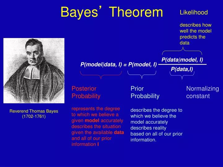
P(data|model, I). P(model|data, I) = P(model, I). P(data,I). Likelihood describes how well the model predicts the data. Bayes ’ Theorem. Posterior Probability represents the degree to which we believe a given model accurately describes the situation

E N D
P(data|model, I) P(model|data, I) = P(model, I) P(data,I) Likelihood describes how well the model predicts the data Bayes’ Theorem Posterior Probability represents the degree to which we believe a given model accurately describes the situation given the available data and all of our prior information I Prior Probability describes the degree to which we believe the model accurately describes reality based on all of our prior information. Normalizing constant Reverend Thomas Bayes (1702-1761)
ml mapping From: Olga Zhaxybayeva and J Peter Gogarten BMC Genomics 2002, 3:4
ml mapping Figure 5. Likelihood-mapping analysis for two biological data sets. (Upper) The distribution patterns. (Lower) The occupancies (in percent)for the seven areas of attraction. (A) Cytochrome-b data fromref. 14. (B) Ribosomal DNA of major arthropod groups (15). From: Korbinian Strimmer and Arndt von HaeselerProc. Natl. Acad. Sci. USAVol. 94, pp. 6815-6819, June 1997
(a,b)-(c,d) /\ / \ / \ / 1 \ / \ / \ / \ / \ / \/ \ / 3 : 2 \ / : \ /__________________\ (a,d)-(b,c) (a,c)-(b,d)Number of quartets in region 1: 68 (= 24.3%)Number of quartets in region 2: 21 (= 7.5%)Number of quartets in region 3: 191 (= 68.2%)Occupancies of the seven areas 1, 2, 3, 4, 5, 6, 7: (a,b)-(c,d) /\ / \ / 1 \ / \ / \ / /\ \ / 6 / \ 4 \ / / 7 \ \ / \ /______\ / \ / 3 : 5 : 2 \ /__________________\ (a,d)-(b,c) (a,c)-(b,d)Number of quartets in region 1: 53 (= 18.9%) Number of quartets in region 2: 15 (= 5.4%) Number of quartets in region 3: 173 (= 61.8%) Number of quartets in region 4: 3 (= 1.1%) Number of quartets in region 5: 0 (= 0.0%) Number of quartets in region 6: 26 (= 9.3%) Number of quartets in region 7: 10 (= 3.6%) Cluster a: 14 sequencesoutgroup (prokaryotes) Cluster b: 20 sequencesother Eukaryotes Cluster c: 1 sequencesPlasmodium Cluster d: 1 sequences Giardia
Li pi= L1+L2+L3 Ni pi Ntotal Alternative Approaches to Estimate Posterior Probabilities Bayesian Posterior Probability Mapping with MrBayes(Huelsenbeck and Ronquist, 2001) Problem: Strimmer’s formula only considers 3 trees (those that maximize the likelihood for the three topologies) Solution: Exploration of the tree space by sampling trees using a biased random walk (Implemented in MrBayes program) Trees with higher likelihoods will be sampled more often ,where Ni - number of sampled trees of topology i, i=1,2,3 Ntotal – total number of sampled trees (has to be large)
Illustration of a biased random walk Figure generated using MCRobot program (Paul Lewis, 2001)
COMPARISON OF DIFFERENT SUPPORT MEASURES A: mapping of posterior probabilities according to Strimmer and von Haeseler B: mapping of bootstrap support values C: mapping of bootstrap support for embedded quartets from extended datasets (see fig. 2) Zhaxybayeva and Gogarten, BMC Genomics 2003 4: 37
Boostrap Support Values for Embedded Quartets vs. Bipartitions: Performance evaluation using sequence simulations and phylogenetic reconstructions
C C C D D D 0.01 0.01 N=8(4) N=4(0) N=5(1) 0.01 A 0.01 0.01 B B A B B A C C D C D D A A B A B B N=13(9) N=23(19) N=53(49)
Methodology : Input tree Aligned Simulated AA Sequences (200,500 and 1000 AA) Seq-Gen WAG, Cat=4 Alpha=1 Seqboot 100 Bootstraps ML Tree Calculation FastTree, WAG, Cat=4 Repeat 100 times Extract Highest Bootstrap support separating AB><CD Consense Extract Bipartitions For each individual trees Count How many trees embedded quartet AB><CD is supported
Results : Maximum Bootstrap Support value for Bipartition separating (AB) and (CD) Maximum Bootstrap Support value for embedded Quartet (AB),(CD)
Vincent Daubin and Howard Ochman: Bacterial Genomes as New Gene Homes: The Genealogy of ORFans in E. coli. Genome Research 14:1036-1042, 2004 The ratio of non-synonymous to synonymous substitutions for genes found only in the E.coli - Salmonella clade is lower than 1, but larger than for more widely distributed genes. Fig. 3 from Vincent Daubin and Howard Ochman, Genome Research 14:1036-1042, 2004
Trunk-of-my-car analogy: Hardly anything in there is the is the result of providing a selective advantage. Some items are removed quickly (purifying selection), some are useful under some conditions, but most things do not alter the fitness. Could some of the inferred purifying selection be due to the acquisition of novel detrimental characteristics (e.g., protein toxicity, HOPELESS MONSTERS)?
sites model in MrBayes The MrBayes block in a nexus file might look something like this: begin mrbayes; set autoclose=yes; lset nst=2 rates=gamma nucmodel=codon omegavar=Ny98; mcmcp samplefreq=500 printfreq=500; mcmc ngen=500000; sump burnin=50; sumt burnin=50; end;
MrBayes analyzing the *.nex.p file • The easiest is to load the file into excel (if your alignment is too long, you need to load the data into separate spreadsheets – see here execise 2 item 2 for more info) • plot LogL to determine which samples to ignore • for each codon calculate the the average probability (from the samples you do not ignore) that the codon belongs to the group of codons with omega>1. • plot this quantity using a bar graph.
the same after rescaling the y-axis plot LogL to determine which samples to ignore
copy paste formula enter formula for each codon calculate the the average probability plot row
To determine credibility interval for a parameter (here omega<1): Select values for the parameter, sampled after the burning. Copy paste to a new spreadsheet,
Sort values according to size, • Discard top and bottom 2.5% • Remainder gives 95% credibility interval.
hy-phy Results of an anaylsis using the SLAC approach
Hy-Phy -Hypothesis Testing using Phylogenies. Using Batchfiles or GUI Information at http://www.hyphy.org/ Selected analyses also can be performed online at http://www.datamonkey.org/
Example testing for dN/dS in two partitions of the data --John’s dataset Set up two partitions, define model for each, optimize likelihood
Example testing for dN/dS in two partitions of the data --John’s dataset Alternatively, especially if the the two models are not nested, one can set up two different windows with the same dataset: Model 1 Model 2
Example testing for dN/dS in two partitions of the data --John’s dataset Simulation under model 2, evaluation under model 1, calculate LR Compare real LR to distribution from simulated LR values. The result might look something like this or this
Other ways to detect positive selection Selective sweeps -> fewer alleles present in population (see contributions from Archaic Humans for example) Repeated episodes of positive selection -> high dN
Necessary assumptions: • Genes are transferred horizontally • (in addition to vertical transmission) • B) Many genes encode weakly selected functions (wsf). • (Examples are • degradation of substrates that are only temporarily present in the environment, • biosynthetic pathways yielding products that frequently are present in the environment, • transport functions related to either of the two processes) • C) If an organism is grown under non-selective conditions, these functions may be lost due to mutations. • If several genes are required for this function, once one of these genes is lost, the others are no longer under any selective pressure, and rapidly accumulate mutations. • Horizontal gene transfer can safe wsf from extinction • When only parts of the genomes are transferred, clustered genes (and the encoded function) are more likely than unclustered genes to be transferred horizontally, .
GENOMES OF CLOSELY RELATED ORGANISMS: CORE AND SHELL core Strain-specific Normand et al, Genome Research 17, 7-15 2007 Dispensable Edwards-Venn cogwheel A.W.F. Edwards 1998 Dispensable Image source: web.uconn.edu/mcbstaff/benson/Frankia/FrankiaHome.htm
Alternatives to selfish operons Horowitz's idea (another great and simple, but wrong ideas; one of the most falsified theories ever) Operons reflect the evolution of biochemical pathways (Extension of Grannik's hypothesis: biosynthesis recapitulates biogenesis )
Horowitz's idea (another great and simple, but wrong ideas; one of the most falsified theories ever) Support: Gene order often reflects order of biochemical reactions. Gene families that originated through duplication often form clusters in eukaryotes (e.g. mammalian beta-globin gene cluster, histones) Problems: Neighboring genes in prokaryotes usually did not result from gene duplications. Gene families that evolved through duplications usually are not neighbors or even part of the same biochemical pathway. E.g.; NAD binding dehydrogenases (GAP, alcohol, lactate and malate DH) are homologous but are part of different pathways and operons.
(Fisher model) Gene clusters evolve through selective advantage due to co-adaptation Enzymes A and B can be present as type A or a and B and b. If AB and ab provide a selective advantage over aB and Ab, and frequent recombination occurs to disrupt co-adapted alleles then close neighborhood of AB decreases the frequency of disruption of co-adapted alleles. Problems Enzymes in metabolic pathways often do not physically interact with each other; Source for frequent recombination unclear.
Operons allow for efficient regulation Pardee, Jacob, Monod model Problems While co-regulation is a definite advantage, this model does not suggest a plausible series of intermediate steps that would give rise the evolution of gene clusters! An advantage is only realized when two genes are actually co-transcribed, not when they move closer to each other. To provide an advantage one needs to assume that one of the genes was inefficiently regulated, while the other one was not. This process needs to be iterated for every gene added to the operon. Several co-regulated genes exist that are not part of a single operon. Gene products encoded as part of the same operon often are needed in different quantities due to different catalytic efficiencies, and SU stoichiometries different from 1:1).
Problems of the selfish operon theory: Not only wsf but most essential genes are clustered Example: ATPsynthase, ribosomal proteins Possible Solution: Horizontal transfer occurs. Co-adaptation (modified Fischer model) would provide an advantage to coadapted SU to be transferred together. The non-coadapted SU that are replaced do not need to be clustered together. Supporting this explanation is the fact the essential functions encoded in operons are structurally interacting.
Problems of the selfish operon theory: Some non-essential genes are not clusteredNot clustered in Salmonella: Cysteine and Methionine biosynthesis pathways Possible explanation: These amino acids are needed in higher amounts than present in the environment because they participate in additional cellular metabolic pathways (SAM, reduced sulfur). These are not wsf.
Problems of the selfish operon theory: Genes are clustered in some species but not in others. Selection pressures different (some bacteria might live in environments that provide sufficient amounts of some metabolites (e.g. purine, nicotine, or thiamine). Benefits due to co-adaptation might be restricted to closely related species (tRNA clusters / codon bias)
Problems of the selfish operon theory: Some operons contain apparently unrelated genes Small deletions will sometimes fuse unrelated genes. These can persist, if they are not counter selected (similar regulation or constitutive expression) Example: polycistronic mRNAs in nuclear rest bodies (nucleomorphs) of cryptophytes and chlorarachniophyta (eukaryotic algae as endosymbionts, nucleus of endosymbiont greatly reduced)