Download
1 / 61
610 likes | 966 Views
Implementation and Statistical Analysis of a Differential GPS System. Team Members: Jim Connor Jon Kerr. Advisor: Dr. In Soo Ahn. Abstract.

E N D
Implementation and Statistical Analysis of a Differential GPS System Team Members: Jim Connor Jon Kerr Advisor: Dr. In Soo Ahn
Abstract • Normal GPS (Global Positioning System) is not accurate enough for the applications here at Bradley University. For greater accuracy, a Differential GPS system will be implemented. To do this, two GPS units are required. A base station, with a known position, sends error correction data to a mobile unit. The error correction data is sent wirelessly through a radio link. The data can then be viewed on a laptop computer for statistical analysis.
Project Purpose • Previous project: Autonomous Vehicle with GPS Navigation - Jason Seelye and Bryan Everett • Problem: GPS not accurate enough to control vehicle • Our focus: Create GPS system with the greatest accuracy possible for the control of autonomous vehicles (sidewalk)
Topics of Discussion • Explanations and Terminology • Equipment used • Project description • Hardware implementation process • Software implementation process • Problems encountered and solutions • Data gathering • Statistical Analysis of data • Conclusions and Recommendations
Explanations and Terminology • Global Positioning System (GPS) – A satellite navigation system capable of providing highly accurate position, velocity, and timing information. • Differential Global Positioning System (DGPS) – A GPS system that is capable of being more accurate by taking into account position correction information. • Circular Error Probability (CEP) – Radius of the circle, centered at the known antenna position, that contains 50% of the data points in a horizontal scatter plot. • Dilution of Precision (DOP) – Accuracy of position due to satellite geometric positions.
Equipment Used • Two NovAtel® RT-20 Receivers • Operate at 1575.42 MHz • 12 Channel Receivers • Two FreeWave® Radios • Operate at 928 MHz • 20 mile line of sight range • NEC® Laptop Computer
Block Diagram Transmitter / Base Station Position Error Corrections GPS Antenna NovAtel Receiver FreeWave Radio Antenna Receiver / Mobile Station Position Error Corrections FreeWave Radio NovAtel Receiver Laptop Computer for analysis Antenna GPS Antenna
Block Diagram Binary data stream Reference Station RF modem RF modem Mobile Station Commands Data Computer Matlab
Functional Description • An exact geographical position is determined. • Reference station placed at this point. • Since at a known position, able to calculate errors from GPS satellites. • Sends error corrections across a wireless radio link to remote station. • Remote station receives error corrections and also position information from same satellite constellation that reference station sees. • Remote station uses both satellite data and error corrections to calculate position. Serial Correction Data NovAtel® Receiver Base Station NovAtel® Receiver Remote Station
Errors Removed by Differential GPS • Ionosphere 0-30 meters Mostly Removed • Troposphere 0-30 meters All Removed • Signal Noise 0-10 meters All Removed • Ephemeris Data 1-5 meters All Removed • Clock Drift 0-1.5 meters All Removed • Multipath 0-1 meters Not Removed • SA 0-70 meters All Removed
Design Approach • Correct operation of NovAtel receivers borrowed from CAT • Correct operation of FreeWave Radio communication link borrowed from Dr. Sennott (TISI) • Successful GPS receiver – radio link integration
Hardware Implementation Reference Point • Placed NovAtel GPS Receiver on Jobst Hall and collected position information (scatter plot) for about two hours. • Used the average Latitude and Longitude of this plot as our reference point.
Hardware Implementation Latitude = 40 41 56.613512 N Longitude = 89 37 1.613741 W Height = 192.341 m
Hardware Implementation Configure Reference Station • Data rate – 9600 bps • Minimum rate – 2400 bps • Fix position of NovAtel reference station. fix position 40.69903722, -89.61712110, 192.3415 • Log differential corrections. log com1 rtcm3 ontime 1 log com1 rtcm59 ontime 1 log com1 rtcm1 ontime 1
RTCM Corrections • Radio Technical Commission for Maritime Services (RTCM) set up a team composed of representatives of US federal authorities, GPS manufacturers and users. • In early 1990, they adopted a first standard for the transmission format and contents for DGPS applications • Special Committee 104 (SC104)
Types of RTCM Log Commands (Access to carrier phase)
Hardware Implementation Configure Mobile Station • Accept differential corrections from reference station accept com2 rt20 • Log GPS data log com1 p20a ontime 1 log com1 dopa ontime 1
Hardware Implementation Saving GPS Data • Using Windows HyperTerminal, save all data to a Notepad file. • Process data in Matlab.
Software Implementation Approach • Use Matlab to read a log file and process data • Plot data points in a scatter plot • Calculate CEP • Plot drifting of position accuracy • Plot position accuracy vs. number of satellites available
Software Flow Chart Open and read log file Convert latitude and longitude to local coordinates (meters) Calculate CEP Plot graphs Calculate and display mean values
Software Implementation Opening and reading log file • R = input('What type of log file is it? 1=POSA 2=P20A 3=P20A and DOPA ') • file = INPUTDLG('Enter the File name','Enter GPS log file to open') • [time lat long height] = textread(file, ' %*s %f %*[^\n]', 'delimiter',',')
Software Implementation Coordinate conversion • Local (North, East, Down) • Uses a reference point to find the change in direction • Converts to meters
Software Implementation Coordinate conversion • lat_ref=mean(lat) long_ref=mean(long) height_ref=mean(height) a = earth_shape; north = (a(2) * (lat - lat_ref))*pi/180; d = a(2) * sin(lat); c = a(1) * cos(lat); lat_angle = atan2(d,c); east = -(a(1) * cos(lat_angle).*(long – long_ref))*pi/180; down = -(height-height_ref);
Software Implementation Calculating CEP • Find the radius of a circle where half of the points lie • Finds distances for all the points • Compares to a incrementing radius • Radius increments in millimeters starting at 1 mm
Software Implementation Calculating CEP
Software Implementation Plotting graphs • Scatter plot plot(east,north,'x'),title('CEP') axis equal • Subplots subplot(311),plot(east),title('East Coordinates'), subplot(312),plot(north),title('North Coordinates'), subplot(313),plot(height),title('Height')
Software Implementation Displaying mean values • 40.69896654 -89.61670040 to • 40° 41’ 56.28”N 89° 37’ 0.11” W • if(lat_ref>0) dirLat='N';else dirLat='S';end lat_ref=abs(lat_ref); deg=floor(lat_ref); min=(lat_ref-deg)*60; sec=(min -floor(min))*60; Lat=sprintf(' %d %d %f %c',deg,floor(min),sec,dirLat);
Problems Encountered • CAT NovAtel receiver missing software • Radio transmitter link doesn’t work or transmit data when connected to GPS receiver • Can’t find geographic benchmark data
Problems Encountered • Transmitter doesn’t transmit data when connected to GPS receiver • Solution • Null-modem/ Straight cable hardware conflict • Bought Null Modem adapter from Radio Shack
Initial Data Gathering Procedure • Set up base station • Set up remote station far away • Start sending corrections • Use laptop to capture remote station data • Process in Matlab CEP = 112 m
Initial Data Gathering Stand alone mode: CEP = 112 m
Initial Data Gathering Differential GPS mode: CEP = 94 m
Initial Data Gathering Ashtech: CEP = 2.6 m
Code Problem • We were converting Latitude and Longitude to meters without first converting to radians • All our conversions were off by a factor of about 57 • 1 radian = 57.3 degrees
Data Gathering Corrected Matlab Code: CEP = 2.07 m
Data Gathering Differential: CEP = 10.7 cm
Data Gathering Differential Steady State: CEP = 4.7 cm
Statistical Analysis • Scatter Plots - CEP • Satellite Switching • Steady State response • DOP • Warm and Cold Start • DGPS – GPS comparison
Statistical Analysis DGPS system operating • CEP • Satellite effects • Time to steady state
Statistical Analysis CEP= 12.7cm 16 min
Steady State Response CEP= 4.7cm
Statistical Analysis DGPS system operating • Fix base station position with less accuracy • What are the effects?
Statistical Analysis CEP = 40cm 30 min
Statistical Analysis Good DOP values are between 1 and 3. Higher values mean poor position accuracy due to spacing of satellites.
Statistical Analysis DOP:
Statistical Analysis DGPS system operating • What are the effects of taking GPS data at warm and cold starts? • Cold start: Initial startup • Warm start: Been running for a while
Statistical Analysis (cold) CEP= 1.83m
Statistical Analysis (warm) CEP= 1.05m