Download
1 / 35
440 likes | 779 Views
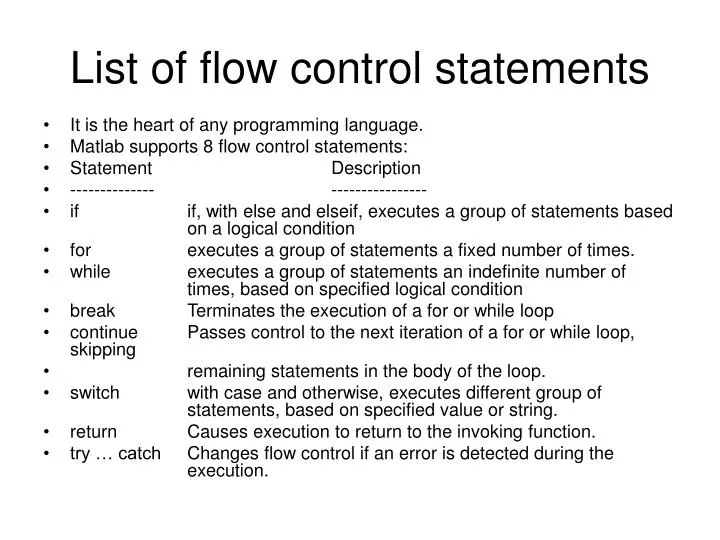
List of flow control statements. It is the heart of any programming language. Matlab supports 8 flow control statements: Statement Description -------------- ---------------- if if, with else and elseif, executes a group of statements based on a logical condition

E N D
List of flow control statements • It is the heart of any programming language. • Matlab supports 8 flow control statements: • Statement Description • -------------- ---------------- • if if, with else and elseif, executes a group of statements based on a logical condition • for executes a group of statements a fixed number of times. • while executes a group of statements an indefinite number of times, based on specified logical condition • break Terminates the execution of a for or while loop • continue Passes control to the next iteration of a for or while loop, skipping • remaining statements in the body of the loop. • switch with case and otherwise, executes different group of statements, based on specified value or string. • return Causes execution to return to the invoking function. • try … catch Changes flow control if an error is detected during the execution.
If statment • if expression • statements • end • The expression is evaluated and if it is true, the statements between if and end are executed otherwise the statements after the end line are executed. • When nesting ifs, each if must be paired with a matching end.
If-elseif-else statement • if expression1 • statements1 • elseif expression2 • statements2 • else • statements3 • end • Here if expression1 is true, the statements1 are executed and then control is transferred to the end statement. • If expression1 is false, the expression2 is evaluated. • If it is true, then statements2 are executed and control is transferred to end statement. • Otherwise statement3 is executed. • Else and elseif appear after an if statement; • They do not need to appear in pairs.
Example for if-elseif-else statements • >> i=6; j=21; • >> if i > 5 • k =i; • elseif (i>1) & (j==20) • i = 5*i+j; • else • k=1; • end • >> k • k =6
For loop It executes a group of statements a specified number of times. The syntax is: • for index = start1:increment1:end • statements1 • for index2 = start2:increment2:end • statements2 • end • additional loop statements • end • count =0; • for k = 0:0.1:1 • count = count + 1; • end • This loop is executed 11 times. If the loop increment is omitted, it is taken to be 1. Loop increments can also be negative. No semicolon is needed at the end of a for loop. Matlab automatically suppresses printing the values of a loop index.
Example of For loop • >> for n=100:-20:0 • k = 1/(exp(n)); • end • >> for n=100:-20:0 • k= 1/(exp(n)); • disp(k) • end • 3.7201e-044 • 1.8049e-035 • 8.7565e-027 • 4.2484e-018 • 2.0612e-009 • 1
While loop • This loop is used to execute a statement or a group of statements for an indefinite number of times until the condition specified by while is no longer satisfied. While loops can also be nested. A while must have a matching end. • while expression • statements • end • a = 10; • b = 5; • while a • a = a -1; • while b • b = b -1; • end • end • Here a numerical values is treated as true when it is nonzero and as false when it is 0.
Example for while loop • >> v = 1; num =1; i =1; • while num < 1000 • num = 2^i; • v = [v; num]; • i = i + 1; • end • >> v • v = 1 • 2 • 4 • 8 • 16 • 32 • 64 • 128 • 256 • 512 • 1024
Break and continue statments • It terminates the execution of a for or while loop. • When it is encountered, execution continues with the next statement outside the loop. • In nested loops, break exits only from the innermost loop that contains it. • Continue • It passes control to the next iteration of the “for or while” loop in which it appears, skipping any remaining statements in the body of the loop. • In nested loops, continue passes control to the next iteration of the loop enclosing it.
Switch case statement • Here a flag (any variable) is used as a switch and the values of the flag make up different cases for execution. • switch flag • case value1 • statement1(s) • case value2 • statement2(s) • otherwise • statement(s) • end • Here statement1(s) are performed if flag=value1, statement2(s) are performed if flag=value2, and so on. If the value of flag does not match any case then the last block computation is done. • Switch can be a numeric variable or a string variable.
Example for switch case • Let us assume that we read the value of the variable ‘newclass’ and convert the image f according to its value. • f=imread(‘cameraman.tif’); • newclass=input(‘newclass=’,’s’); • switch newclass • case ‘uint8’ • g = im2uint8(f); • case ‘uint16’ • g = im2uint16(f); • case ‘double’ • g = im2double(f); • otherwise • error(‘Unknown image class’) • end
Compiled (Parsed) functions: P-Code When a function is executed in Matlab, each command in the function is first interpreted by Matlab and then translated into the lower level language. This process is called parsing. It is not exactly like compiling in C, but is a similar process. To parse a function called proj, that exists in an M-file called proj.m, type the command • pcode proj • This command generates a parsed function that is saved in a file named proj.p. • Next time when we call the function proj, Matlab directly executes the preparsed function. • The best use of p-codes, is in protecting our proprietary rights when we send our functions to other people. • We can send the p-codes, the recipients can execute them but they cannot modify them.
Profiler • It keeps track of the time spent on each line of the function (in units of 0.01 seconds) as the function is executed. • The profiler report show how much time is spent on which line. • The command ‘profile on’turns the profiler. • The command ‘profile report’ show the profiler report. • The command ‘profile plot’ show the report as a pareto plot. • The command ‘profile done’ closes the profiler. • The profiler can be used only on functions (not scripts) and those functions that exist as M-files.
Inline functions • To define simple functions one can use inline functions – the functions that are created on the command line. • The syntax is: F = inline(‘function formula’) • >> fx = inline(‘x^2 + sin(x)’) • >> fx(pi) • Or • >> x = [ 0 pi/4 pi/2 3*pi/4 pi] • >>fx(x) • Or • sin(fx(0.5))
Error() and menu() • The command error(‘message’) inside a function or a script aborts the execution, displays the error message and returns the control to the keyboard. • The command menu(‘Menuname’, ‘option1’,’option2’,…) creates an on-screen menu with the Menuname and lists the options in the menu. • User can select any options using mouse or keyboard
Example for menu • >> %plotting a circle • r = input('enter the radius'); • theta = linspace(0, 2*pi, 100); • r = r*ones(size(theta)); • coord= menu('circleplot','cartesian','polar'); • if coord==1 • plot(r.*cos(theta), r.*sin(theta)) • axis('square') • else • polar(theta,r); • end
Plotting in Matlab • The Matlab commands used for plotting are: • plot creates a 2-D line plot • axis changes the aspect ratio of x & y axes • xlable annotates the x-axis • ylable annotates the y-axis • title puts a title on the plot • print prints a hardcopy of the plot
Example for plotting • >> theta = linspace(0,2*pi,100); • x = cos(theta); • y = sin(theta); • plot(x,y) • axis('equal'); • xlabel('x') • ylabel('y') • title('Circle of unit radius')
Multiple plots • Text strings are entered within single right-quote characters. • To display the data points with small circles, use plot (x,y,’o’). • We can combine the two plots with the command plot(x,y,x,y,’o’) to show the line through the data points as well as the distinct data points. • To overlay plots: We can use plot(x,y,x,z,’—‘) or we can plot the first curve, use the hold on command, and then pot the second curve on top of the first one. • plot(xdata,ydata) produces a plot with xdata on the horizontal axis and ydata on the vertical axis. • The important thing to remember about the plot command is that the vector inputs for the x-axis and y-axis data must be of the same length.
fplot • fplot takes the function of a single variable and the limits of the axes as the input and produces a plot of the function. • fplot(‘function’, [xmin xmax]) • >> fplot('exp(-0.1*x)*sin(x)', [0, 20]) • ezplot3 : It takes 3 input arguments to plot the 3D parametric curves • >> x = 't.*cos(3*pi*t)'; y = 't.*sin(3*pi*t)'; z = 't'; • >> ezplot3(x,y,z) • ezcontour plots contour of a given function • ezsurf produces the 3D surface plots.
Cell arrays • When dealing with mixed variables (characters and numbers), we use cell array. • A cell array is a multidimensional array whose elements are copies of other arrays. (eg) • c = { ‘gauss’, [ 1 0; 0 1], 3} • contains 3 elements: a character string, a 2 X 2 matrix and a scalar. Note that we use curly braces for cell array. • To select the contents of a cell array, we enclose an integer address in curly braces. • >> c{1} • ans = gauss • >> c{2} • ans = 1 0 0 1 • >> c{3} • ans = 3. • Cell array contain copies of arguments, not pointers to the arguments.
Structures • Structures are similar to cell arrays, allow grouping of a collection of dissimilar data into a single variable. • Elements of structures are addressed by names called fields. • Let S denote the structure variable and using the (arbitrary) field names char_string, matrix, and scalar, the data in the above example can be accessed using: • S.char_string = ‘gauss’; • S.matrix = [ 1 0; 0 1]; • S.scalar = 3; • The dot operator append the various fields to the structure variable. • >> S.matrix • ans = 1 0 0 1
Script File • A script file is user-created file with a sequence of Matlab commands in it. • The file name must be saved with a .m extension to its name, making it an M-file. • It is useful, when we have to repeat a set of commands several times. • A script file is executed by typing its name (without the .m extension) at the command prompt. • Script files work on global variables. • Results obtained from executing script files are left in the workspace. • If we want to do a big set of computations but in the end we want only a few outputs, a script file is not the good choice.
Example for script file • The lines starting with a % sign are interpreted as comment lines by Matlab and are ignored. • % Circle – A script file to draw a unit circle • % File written by K.Ganesan on 10/12/2007 • % ------------------------------------------------- • theta = linspace(0,2*pi,100); • x = cos(theta); • y = sin(theta); • plot(x,y); • axis(‘equal’); • title(‘Circle of unit radius’);
Invoking a script file • Let us type the above set of Matlab commands in an editor and store it in a file called circle.m. • Then when we type ‘help circle’ in the command window the comment statements of circle file are displayed. • To execute the above file, we type circle. • The contents of an m file can be displayed using : • >>type circle.m • To get an input from the user use ‘input’: • >>x= input(‘Enter the radius of the circle’); • To display the value of a variable, we can use • >>disp(x);
Functions • A function file is also an M-file, like a script file, except that it has a function definition line, which defines the input and output explicitly. • Functions can have arguments, script files do not. • The variables in a function file are all local. • To check if a function or script file of the proposed name already exist, we use: exist(‘fname’); • which returns zero if nothing with name fname exists.
Example for function • function [x, y] = circlefn(r); • %CIRCLEFN – Function to draw a circle of radius r • %Call syntax: [x, y] = circlefn(r) or circlefn(r); • %Input: r = given radius Output: [x,y] = x and y coordinates of data points • theta = linspace(0, 2*pi, 100); • x = r*cos(theta); • y = r*sin(theta); • plot(x,y); • axis(‘equal’); • title([‘Circle of Radius = ‘, num2str(r)]) • Save this file as circlefn.m. • Usually Matlab automatically writes the name of the function as the file name.
Invoking a function • To execute the above function, we can use: • >> r =8; • >> [x,y] = circlefn(8); • or • >> [resx, resy] = circlefn(4.5); • or • >> circlefn(3); • The function feval evaluates a function whose name is specified as a string at the given list of input variables. • (eg) [y, z] = feval(‘circlefn’, r); evaluates the function circlefn on the input variable r and returns the output in y and z. It is equivalent to typing: [y z] = circlefn(r). • >> [y, z] = feval('circlefn', 4.5); • All functions written below the first function in the file are called as subfunctions and they are NOT available to the outside world.
File handling in Matlab • Matlab supports many standard C language file I/O functions for reading and writing formatted binary and text files. Some important functions are: • fopen - Opens an existing file or creates a new file • fclose - Closes an open file • fread - Reads binary data from a file • fwrite - Writes binary data to a file • fscanf - Reads formatted data from a file • fprintf - Writes formatted data to a file • sscanf - Reads strings in specified format • sprintf - Writes data in formatted string • fgets - Reads a line from file discarding new-line character • fgetl - Reads a line from file including the new-line character • frewind - Rewinds a file • fseek - Set the file position indicator • ferror - Inquires file I/O error status.
Example of file handling • % TEMPTABLE – generates and stores temperature data • % Script file • f = -40:5:100; • c = (f-32)*5/9; • t = [f;c]; • fid = fopen('temp.table','w'); • fprintf(fid, ' Temperature table\n'); • fprintf(fid, ' ---------------------\n '); • fprintf(fid, 'Farenheit Celsius\n'); • fprintf(fid, ' %4i %9.3f\n',f); • fclose(fid); • Here ‘fopen’ opens a file in the write mode (‘w’) and assigns the file identifier to fid. In fprintf command, %4i stands for an integer field of width 4 and %8.2f stands for a fixed point field of width 8 with 2 digits after the decimal point.
Other useful Matlab commands • The command pause temporarily halts the current process. pause(n) halts the current process for n seconds. Pressing any key can resume the process. • Importing data files • One can import different types of data files, using a GUI and command line. • >> uiimport temp.table % here temp.table is the name of the file to be imported. • Here the file format can be a text data, spreadsheet data, movie data, image data or audio data. We can also import data from a file using the built-in-function • importdata(filename)
Some useful commands • Saving and loading data • Mat-files are written in binary format with full 16-bit precision. It is possible to write data in 8-digit or 16-digit ASCII format with the optional arguments to the save command. The data saved in these files can be loaded into the Matlab using load command. • save out.dat x –ascii (saves variable x in the file out.dat in 8-digit ascii format) • load out.dat (loads the variables saved in the file out.dat) • Eigenvalue of a matrix A, can be obtained using eig(A) • >> A = [5 -3 -2; -3 8 4; 4 2 -9]; • >> eig(A) • >> [eigvec, eigval] = eig(A) • Here eigvec gets the eigenvectors of A. • Determinant of a matrix • >>det(A) is the determinant of the square matrix A.
Interactive Computation • If our command is too long to fit into one line, then type three periods continuously at the end of the first line. • Our command can be up to 4096 characters long. • Internally computations are done in double precision. • We can use diary command and save our entire session in it. • We can specify the name of the file in which we want to record our session. • It can be invoked using ‘diary on’ command and terminated using ‘diary off’ command.
Example for diary • >> diary 'session' % name of the file in which we want to save our sessions • >> diary on % switching the diary operation • >> disp('good morning'); % activity to be recorded • >> disp(‘Matlab is excellent’); • >> disp(‘You can do wonderful things in Matlab’); • >> diary off % switching the diary off • >> type session % playing the contents of diary
Function input • Function input is used for inputting data into an M-function. The syntax is: • t = input(‘message’) • This function outputs the words contained in message and waits for an input from the user, followed by a return and stores the input in t. • The input can be a number, a string, a vector, a matrix or other valid MATLAB data structure. • >>t = input(‘ Enter your data:’, ‘s’) • This command output the content ‘Enter your data:’ and accepts a character string.