Download
1 / 37
1.78k likes | 3.92k Views
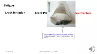
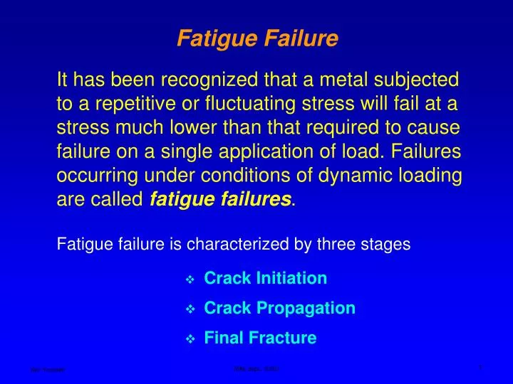
Fatigue failure is characterized by three stages. Crack Initiation. Crack Propagation. Final Fracture. Fatigue Failure.

E N D
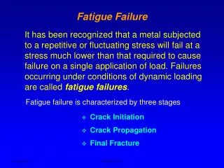
Fatigue failure is characterized by three stages • Crack Initiation • Crack Propagation • Final Fracture Fatigue Failure It has been recognized that a metal subjected to a repetitive or fluctuating stress will fail at a stress much lower than that required to cause failure on a single application of load. Failures occurring under conditions of dynamic loading are called fatigue failures. MAE dept., SJSU
Crack initiation site Fracture zone Propagation zone, striation Jack hammer component, shows no yielding before fracture. MAE dept., SJSU
VW crank shaft – fatigue failure due to cyclic bending and torsional stresses Propagation zone, striations Crack initiation site Fracture area MAE dept., SJSU
928 Porsche timing pulley Crack started at the fillet MAE dept., SJSU
Fracture surface of a failed bolt. The fracture surface exhibited beach marks, which is characteristic of a fatigue failure. 1.0-in. diameter steel pins from agricultural equipment. Material; AISI/SAE 4140 low allow carbon steel MAE dept., SJSU
bicycle crank spider arm This long term fatigue crack in a high quality component took a considerable time to nucleate from a machining mark between the spider arms on this highly stressed surface. However once initiated propagation was rapid and accelerating as shown in the increased spacing of the 'beach marks' on the surface caused by the advancing fatigue crack. MAE dept., SJSU
Crank shaft Gear tooth failure MAE dept., SJSU
Hawaii, Aloha Flight 243, a Boeing 737, an upper part of the plane's cabin area rips off in mid-flight. Metal fatigue was the cause of the failure. MAE dept., SJSU
Fracture Surface Characteristics Mode of fracture Typical surface characteristics Ductile Cup and ConeDimplesDull SurfaceInclusion at the bottom of the dimple Brittle Intergranular ShinyGrain Boundary cracking Brittle Transgranular ShinyCleavage fracturesFlat Fatigue BeachmarksStriations (SEM)Initiation sitesPropagation zoneFinal fracture zone MAE dept., SJSU
Alternating stress min max a = 2 Mean stress min max + m= 2 Fatigue Failure – Type of Fluctuating Stresses MAE dept., SJSU
Typical testing apparatus, pure bending Motor Load Rotating beam machine – applies fully reverse bending stress Fatigue Failure, S-N Curve Test specimen geometry for R.R. Moore rotating beam machine. The surface is polished in the axial direction. A constant bending load is applied. MAE dept., SJSU
′ Se Infinite life Finite life S′e = endurance limit of the specimen Fatigue Failure, S-N Curve N > 103 N < 103 MAE dept., SJSU
Steel ′ ′ Se = Se = Sut ≤ 200 ksi (1400 MPa) 0.5Sut Sut> 200 ksi 100 ksi Sut> 1400 MPa 700 MPa Cast iron Cast iron 0.4Sut Sut< 60 ksi (400 MPa) Sut ≥60 ksi 24 ksi Sut< 400 MPa 160 MPa Relationship Between Endurance Limit and Ultimate Strength Steel MAE dept., SJSU
′ ′ Se = Se = Sut < 40 ksi (280 MPa) Sut < 48 ksi (330 MPa) 0.4Sut 0.4Sut Sut ≥ 40 ksi Sut ≥ 48 ksi 14 ksi 19 ksi Sut ≥ 330 MPa Sut ≥ 280 MPa 130 MPa 100 MPa Copper alloys Copper alloys For N = 5x10⁸ cycle Relationship Between Endurance Limit and Ultimate Strength Aluminum Aluminum alloys For N = 5x10⁸ cycle MAE dept., SJSU
′ Se = endurance limit of the specimen (infinite life > 106) Se = endurance limit of the actual component (infinite life > 106) Sf = fatigue strength of the actual component (infinite life > 5x10⁸) S Se ′ Sf = fatigue strength of the specimen (infinite life > 5x10⁸) N 106 103 For materials that do not exhibit a knee in the S-N curve, the infinite life taken at 5x10⁸ cycles S Sf N 5x10⁸ 103 Correction Factors for Specimen’s Endurance Limit For materials exhibiting a knee in the S-N curve at 106 cycles MAE dept., SJSU
′ Se = Cload Csize Csurf Ctemp Crel (Se) • Load factor, Cload Pure bending Cload = 1 Pure axial Cload = 0.7 Pure torsion Cload = 1 if von Mises stress is used, use 0.577 if von Mises stress is NOT used. Combined loading Cload = 1 Correction Factors for Specimen’s Endurance Limit MAE dept., SJSU
d ≤ 0.3 in. (8 mm) Csize = 1 0.3 in. < d ≤ 10 in. Csize = .869(d)-0.097 8 mm < d ≤ 250 mm Csize = 1.189(d)-0.097 Correction Factors for Specimen’s Endurance Limit • Size factor, Csize Larger parts fail at lower stresses than smaller parts. This is mainly due to the higher probability of flaws being present in larger components. For solid round cross section If the component is larger than 10 in., use Csize = .6 MAE dept., SJSU
Correction Factors for Specimen’s Endurance Limit For non rotating components, use the 95% area approach to calculate the equivalent diameter. Then use this equivalent diameter in the previous equations to calculate the size factor. A95 d d95 dequiv = ( )1/2 0.0766 MAE dept., SJSU
Correction Factors for Specimen’s Endurance Limit • surface factor, Csurf The rotating beam test specimen has a polished surface. Most components do not have a polished surface. Scratches and imperfections on the surface act like a stress raisers and reduce the fatigue life of a part. Use either the graph or the equation with the table shown below. Csurf = A (Sut)b MAE dept., SJSU
Correction Factors for Specimen’s Endurance Limit • Temperature factor, Ctemp High temperatures reduce the fatigue life of a component. For accurate results, use an environmental chamber and obtain the endurance limit experimentally at the desired temperature. For operating temperature below 450 oC (840 oF) the temperature factor should be taken as one. Ctemp = 1 for T ≤ 450 oC (840 oF) MAE dept., SJSU
Correction Factors for Specimen’s Endurance Limit • Reliability factor, Crel The reliability correction factor accounts for the scatter and uncertainty of material properties (endurance limit). MAE dept., SJSU
Notch sensitivity factor Kf = 1 + (Kt – 1)q Fatigue Stress Concentration Factor, Kf Experimental data shows that the actual stress concentration factor is not as high as indicated by the theoretical value, Kt. The stress concentration factor seems to be sensitive to the notch radius and the ultimate strength of the material. MAE dept., SJSU
Fatigue Stress Concentration Factor, Kf for Aluminum MAE dept., SJSU
Use the design equation to calculate the size Se Kf a = n Design process – Fully Reversed Loading for Infinite Life • Determine the maximum alternating applied stress, a, in terms of the size and cross sectional profile • Select material → Sy, Sut • Choose a safety factor → n • Determine all modifying factors and calculate the endurance limit of the component → Se • Determine the fatigue stress concentration factor, Kf • Investigate different cross sections (profiles), optimize for size or weight • You may also assume a profile and size, calculate the alternating stress and determine the safety factor. Iterate until you obtain the desired safety factor MAE dept., SJSU
Sn = a (N)b equation of the fatigue line A A S S B B Sf Se Sn = .9Sut N N 106 5x10⁸ 103 103 Point A N = 103 Sn = .9Sut Sn = Se Sn = Sf Point A Point B Point B N = 103 N = 106 N = 5x10⁸ Design for Finite Life MAE dept., SJSU
log .9Sut = loga + blog103 logSe = loga + blog106 (.9Sut)2 Se .9Sut ( ) a 1 = b log .9Sut = Se log ⅓ Se 3 N ( ) Se Sn = 106 Sn Kf a = n CalculateSnand replace Sein the design equation Design equation Design for Finite Life Sn = a (N)b log Sn = log a + b log N Apply conditions for point A and B to find the two constants “a” and “b” MAE dept., SJSU
a Yield line Sy Gerber curve Se Alternating stress Goodman line m Sut Sy Soderberg line Mean stress The Effect of Mean Stress on Fatigue Life Mean stress exist if the loading is of a repeating or fluctuating type. MAE dept., SJSU
a C Safe zone Alternating stress m The Effect of Mean Stress on Fatigue Life Modified Goodman Diagram Yield line Sy Se Goodman line Sut Sy Mean stress MAE dept., SJSU
Safe zone Goodman line - Syc Sut The Effect of Mean Stress on Fatigue Life Modified Goodman Diagram a Sy Yield line Se C Safe zone +m Sy - m MAE dept., SJSU
m > 0 m≤0 Fatigue, Fatigue, Infinite life Se a m 1 a= Finite life = + nf nf a m Se Sut 1 = + Yield Sy Sy Sn Sut a+ m= a+ m= Yield ny ny The Effect of Mean Stress on Fatigue Life Modified Goodman Diagram a Se C Safe zone Safe zone +m Sy Sut - m - Syc MAE dept., SJSU
Calculate the stress concentration factor for the mean stress using the following equation, Kfa Sy Kfm= m Fatigue design equation Kf a Kfmm 1 Infinite life = + nf Se Sut Applying Stress Concentration factor to Alternating and Mean Components of Stress • Determine the fatigue stress concentration factor, Kf, apply directly to the alternating stress → Kfa • If Kf max < Sy then there is no yielding at the notch, use Kfm =Kf and multiply the mean stress by Kfm → Kfmm • If Kf max > Sy then there is local yielding at the notch, material at the notch is strain-hardened. The effect of stress concentration is reduced. MAE dept., SJSU
Calculate the alternating and mean principal stresses, 1a, 2a= (xa /2)± (xa /2)2+ (xya)2 1m, 2m= (xm /2)± (xm /2)2+ (xym)2 Combined Loading All four components of stress exist, xaalternating component of normal stress xmmean component of normal stress xyaalternating component of shear stress xymmean component of shear stress MAE dept., SJSU
a′ = (1a+ 2a - 1a2a)1/2 m′ = (1m+ 2m - 1m2m)1/2 2 2 2 2 ′a ′m 1 = + nf Se Sut Fatigue design equation Infinite life Combined Loading Calculate the alternating and mean von Mises stresses, MAE dept., SJSU
Calculate the support forces, R1 = 2500, R2 = 7500 lb. The critical location is at the fillet, MA = 2500 x 12 = 30,000 lb-in 32M 305577 Mc a= Calculate the alternating stress, = = I πd 3 d 3 Determine the stress concentration factor D r = 1.5 = .1 Kt = 1.7 d d 10,000 lb. Design Example 6˝ 6˝ 12˝ A rotating shaft is carrying 10,000 lb force as shown. The shaft is made of steel withSut = 120 ksi and Sy = 90 ksi. The shaft is rotating at 1150 rpm and has a machine finish surface. Determine the diameter, d, for 75 minutes life. Use safety factor of 1.6 and 50% reliability. d D = 1.5d A R1 R2 r (fillet radius) = .1d m= 0 MAE dept., SJSU
Kf = 1 + (Kt – 1)q = 1 + .85(1.7 – 1) = 1.6 Csurf = A (Sut)b = 2.7(120)-.265 = .759 0.3 in. < d ≤ 10 in. Csize = .869(d)-0.097 = .869(1)-0.097 = .869 Design Example Assume d = 1.0 in Using r = .1and Sut = 120 ksi, q (notch sensitivity) = .85 Calculate the endurance limit Cload = 1 (pure bending) Crel = 1 (50% rel.) Ctemp= 1 (room temp) ′ Se = Cload Csize Csurf Ctemp Crel (Se) = (.759)(.869)(.5x120) = 39.57 ksi MAE dept., SJSU
39.57 ( ) log ⅓ .9x120 86250 ( ) Sn 39.57 = = 56.5 ksi 106 Sn 56.5 305577 n = a= = .116 < 1.6 = = 305.577 ksi Kfa 1.6x305.577 d 3 So d = 1.0 in. is too small Se ( ) .9Sut log ⅓ Assume d = 2.5 in N ( ) Se Sn = All factors remain the same except the size factor and notch sensitivity. 106 Using r = .25and Sut = 120 ksi, q (notch sensitivity) = .9 Kf = 1 + (Kt – 1)q = 1 + .9(1.7 – 1) = 1.63 Se =36.2 ksi → Design Example Design life, N = 1150 x 75 = 86250 cycles Csize = .869(d)-0.097 = .869(2.5)-0.097 = .795 MAE dept., SJSU
Se =36.2 ksi Sn=53.35 ksi → 305577 a= = 19.55 ksi (2.5)3 Sn 53.35 n = = 1.67 ≈ 1.6 = Kfa 1.63x19.55 d=2.5 in. Check yielding Sy 90 n= 2.8 > 1.6 okay = = Kfmax 1.63x19.55 Design Example MAE dept., SJSU